2. Linear Algebra¶

2.1. Introduction¶

Linear Algebra is the study of transformations in vector space. It explains all the relations between points in a given space, position, rotation, distance, velocity, acceleration, and more. As each data point in real-world applications can be represented as a vector, an array of numerals, Linear Algebra is one of the best ways to represent data and is key to Machine Learning.

2.2. Fundamental Objects¶

Scalars, Vectors, and Matrices are the fundamental structures of Linear Algebra. In the section, we introduce each of those objects and their properties.

2.2.1. Scalars¶

Scalars $s$ represent numerical values. Attributes such as the speed of light, the age of a person are scalars.

age = 24    # Age of a person
c = 3e-8    # Celerity of light

2.2.2. Vectors¶

Vectors $\vec{v}$ are arrays or collections of scalars. A component of a vector is referred to as a coordinate, and the number of coordinates corresponds to the dimensionality $d$ of the vector. In 2D space, a point can be represented as a vector $\vec{p}$ with two components $p_x$ and $p_y$. A vector can also be used to represent multiple attributes such as the age and the height of a person. A scalar can be defined as a one-dimensional vector.

\[\begin{split} \vec{v} = \begin{pmatrix} v_1 \\ v_2 \\ \vdots \\ v_n \end{pmatrix} \end{split}\]

Note

Vectors are represented as column vectors by default for convenience (useful for data science).

import numpy as np


coords = np.array([1, -1])      # x, y
person = np.array([24, 175])    # age, height

A vector is often referred to as a geometric vector representing a direction and its magnitude. Each of its components is responsible for the rate of change along its corresponding axis. This kind of vector representation is used in physics to represent an object’s movement with a velocity $\vec{v}$ vector and an acceleration one $\vec{a}$.

import numpy as np
import matplotlib.pyplot as plt
plt.ion()
plt.style.use('fivethirtyeight')

X = np.array([0, 0, 0])
Y = np.array([0, 0, 0])
U = np.array([1, 1, 0])
V = np.array([1, 0, 1])
C = ["r", "g", "b"]

fig = plt.figure(figsize=(4, 4), facecolor="white")
ax = fig.add_subplot(1, 1, 1)

ax.quiver(X, Y, U, V, color=C, units='xy', scale=1)

ax.set_xticks(range(-1, 1 + 1))
ax.set_yticks(range(-1, 1 + 1))
ax.set_xlabel("x")
ax.set_ylabel("y")
ax.set_xlim(-2, 2)
ax.set_ylim(-2, 2)
ax.set_aspect("equal")

fig.canvas.draw()

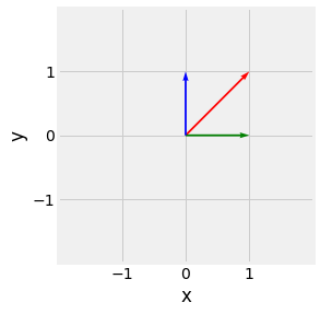
Fig. 2.4 Geometric 2 dimensional vector representation, $\begin{pmatrix}0\\1\end{pmatrix}$ in blue, $\begin{pmatrix}1\\0\end{pmatrix}$ in green, and $\begin{pmatrix}1\\1\end{pmatrix}$ in red.¶

2.2.2.1. Magnitude and Unit Vector¶

For a vector of dimension n, the magnitude (length) is defined as follow:

\[ \|\vec{v}\| = \sqrt{\sum_{i=1}^n v_i^2} \]

A vector with magnitude one is called a unit vector. Any vector can be transformed into its unit equivalent by dividing it by its magnitude:

\[ \vec{u} = \frac{\vec{v}}{\|\vec{v}\|} \]

import numpy as np

def magnitude(v: np.ndarray) -> float:
    return np.sqrt((v ** 2).sum())

v = np.array([1, 1])    # Vector
u = v / magnitude(v)    # Unit Vector

# Casting to float32 for floatting point apporximation errors
magnitude(v).astype(np.float32), magnitude(u).astype(np.float32)

(1.4142135, 1.0)

2.2.2.2. Scaling and Addition¶

A vector can be be multiplied or scaled (thus divided), by any scalar and two vectors of same dimension can be added (thus subsracted) together.

\[\begin{split} \begin{align} s\vec{v} = \begin{pmatrix} sv_1 \\ sv_2 \\ \vdots \\ s.v_n \end{pmatrix} && \vec{u} + \vec{v} = \begin{pmatrix} u_1 + v_1 \\ u_2 + v_2 \\ \vdots \\ u_n + v_n \end{pmatrix} \end{align} \end{split}\]

import numpy as np

s = 1.2                  # Scalar
v = np.array([-2, 5])    # Vector

s * v, v - v

(array([-2.4,  6. ]), array([0, 0]))

import numpy as np
import matplotlib.pyplot as plt
plt.ion()
plt.style.use('fivethirtyeight')

fig = plt.figure(figsize=(8, 4), facecolor="white")
ax1, ax2 = [fig.add_subplot(1, 2, i + 1) for i in range(2)]

X = np.array([0,  0.0])
Y = np.array([0,  0.0])
U = np.array([1, -0.5])
V = np.array([1, -0.5])
C = ["r", "g"]

ax1.quiver(X, Y, U, V, color=C, units='xy', scale=1)

X = np.array([ 0.0,  0.0,  0.0,  1.0, -1.0])
Y = np.array([-1.0, -1.0, -1.0,  1.0, -1.0])
U = np.array([ 1.0, -1.0,  0.0, -1.0,  1.0])
V = np.array([ 2.0,  0.0,  2.0,  0.0,  2.0])
C = ["r", "g", "b", "gray", "gray"]

ax2.quiver(X, Y, U, V, color=C, units='xy', scale=1)

ax1.set_xticks(range(-1, 1 + 1))
ax1.set_yticks(range(-1, 1 + 1))
ax1.set_xlabel("x")
ax1.set_ylabel("y")
ax1.set_xlim(-2, 2)
ax1.set_ylim(-2, 2)
ax1.set_aspect("equal")
ax1.title.set_text("Vector Scaling")

ax2.set_xticks(range(-1, 1 + 1))
ax2.set_yticks(range(-1, 1 + 1))
ax2.set_xlabel("x")
ax2.set_ylabel("y")
ax2.set_xlim(-2, 2)
ax2.set_ylim(-2, 2)
ax2.set_aspect("equal")
ax2.title.set_text("Vector Addition")

fig.subplots_adjust(hspace=0.25, wspace=0.40)
fig.canvas.draw()

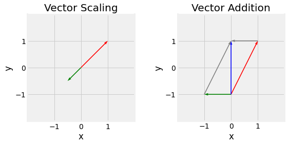
Fig. 2.5 Vector scaling (left) with $s=-0.5$, original vector in red, scaled in green, and Vector addition (right), $\vec{u}$ in red, $\vec{v}$ in green, and $\vec{u}+\vec{v}$ in blue.¶

2.2.2.3. Dot Product¶

The dot (scalar) product of two n-dimensional vectors is defined as follow:

\[ \begin{align} \vec{u}.\vec{v} = \|\vec{u}\| \|\vec{u}\| cos(\theta) && \vec{u}.\vec{v} = \sum_{i=1}^n u_iv_i \end{align} \]

The dot product gives us informations about the angle between two vectors. If $\vec{u}.\vec{v}$ is null, they are perpendicular, also sayed othogonal. Respectively it their dot product is one and both $\vec{u}$ and $\vec{v}$ are unit vectors, they are colinear (pointing in the same direction).

import numpy as np


u = np.array([ 1, 0])
v = np.array([ 0, 1])
w = np.array([-1, 0])

# Perpendicular, Colinear
u.dot(v), u.dot(w)

(0, -1)

import numpy as np
import matplotlib.pyplot as plt
plt.ion()
plt.style.use('fivethirtyeight')

fig = plt.figure(figsize=(12, 4), facecolor="white")
ax1, ax2, ax3 = [fig.add_subplot(1, 3, i + 1) for i in range(3)]

X = np.array([0, 0])
Y = np.array([0, 0])
U = np.array([1 / np.sqrt(np.sum(np.array([1, 1]) ** 2)), -0.3 / np.sqrt(np.sum(np.array([-0.3, 1.0]) ** 2))])
V = np.array([1 / np.sqrt(np.sum(np.array([1, 1]) ** 2)),  1.0 / np.sqrt(np.sum(np.array([-0.3, 1.0]) ** 2))])
C = ["r", "g"]

ax1.quiver(X, Y, U, V, color=C, units='xy', scale=1)
ax1.add_artist(plt.Circle((0, 0), 1.0, color='b', alpha=0.4, fill=False))

X = np.array([0.0,  0.0])
Y = np.array([0.0,  0.0])
U = np.array([1.0, -1.0])
V = np.array([0.0,  0.0])
C = ["r", "g"]

ax2.quiver(X, Y, U, V, color=C, units='xy', scale=1)
ax2.add_artist(plt.Circle((0, 0), 1.0, color='b', alpha=0.4, fill=False))

X = np.array([0.0, 0.0])
Y = np.array([0.0, 0.0])
U = np.array([1.0, 0.0])
V = np.array([0.0, 1.0])
C = ["r", "g"]

ax3.quiver(X, Y, U, V, color=C, units='xy', scale=1)
ax3.add_artist(plt.Circle((0, 0), 1.0, color='b', alpha=0.4, fill=False))

ax1.set_xticks(range(-1, 1 + 1))
ax1.set_yticks(range(-1, 1 + 1))
ax1.set_xlabel("x")
ax1.set_ylabel("y")
ax1.set_xlim(-2, 2)
ax1.set_ylim(-2, 2)
ax1.set_aspect("equal")
ax1.title.set_text("Arbitrary Vectors")

ax2.set_xticks(range(-1, 1 + 1))
ax2.set_yticks(range(-1, 1 + 1))
ax2.set_xlabel("x")
ax2.set_ylabel("y")
ax2.set_xlim(-2, 2)
ax2.set_ylim(-2, 2)
ax2.set_aspect("equal")
ax2.title.set_text("Colinear Vectors")

ax3.set_xticks(range(-1, 1 + 1))
ax3.set_yticks(range(-1, 1 + 1))
ax3.set_xlabel("x")
ax3.set_ylabel("y")
ax3.set_xlim(-2, 2)
ax3.set_ylim(-2, 2)
ax3.set_aspect("equal")
ax3.title.set_text("Orthogonal Vectors")

fig.subplots_adjust(hspace=0.25, wspace=0.40)
fig.canvas.draw()

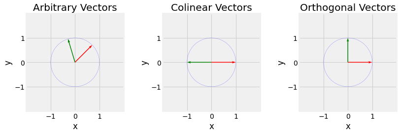
Fig. 2.6 Visualization of arbitrary vectors left, colinear vectors middle, and orthogonal vectors right. Try to visualize the perpendicular projection of the green vector on the red one. In the case of colinear vectors, the length of the new vector obtained by projection is $0$, $-1$ in the case of the colinear vectors (they reflect), and an arbitrary positive number between $0$ and $1$ for the arbitrary one.¶

2.2.2.4. Cross Product¶

In a 3-dimensional euclidean space, the cross product between two vectors is define as follow:

\[\begin{split} \vec{u} \times \vec{v} = \begin{pmatrix} u_y v_z - u_z v_y \\ u_z v_x - u_x v_z \\ u_x v_y - u_y v_x \end{pmatrix} \end{split}\]

The cross product gives birth to a new vector orthogonal to the two others of length $\|\vec{w}\| = \|\vec{u}\| \|\vec{v}\| sin(\theta)$, forming a base $(\vec{u}, \vec{v}, \vec{w})$ with a direction given by the Right-Hand-Rule.

import numpy as np

u = np.array([1, 0, 0])
v = np.array([0, 1, 0])

np.cross(u, v)

array([0, 0, 1])

from mpl_toolkits.mplot3d import Axes3D

import numpy as np
import matplotlib.pyplot as plt
plt.style.use('fivethirtyeight')

X = np.array([0, 0, 0])
Y = np.array([0, 0, 0])
Z = np.array([0, 0, 0])
U = np.array([1, 0, 0])
V = np.array([0, 1, 0])
W = np.array([0, 0, 1])

fig = plt.figure(figsize=(8, 8), facecolor="white")

ax = fig.gca(projection='3d')
ax.quiver(X[0], Y[0], Z[0], U[0], V[0], W[0], color="r")
ax.quiver(X[1], Y[1], Z[1], U[1], V[1], W[1], color="g")
ax.quiver(X[2], Y[2], Z[2], U[2], V[2], W[2], color="b")
ax.patch.set_facecolor('white')
ax.dist = 12

ax.set_xticks(range(-1, 1 + 1))
ax.set_yticks(range(-1, 1 + 1))
ax.set_zticks(range(-1, 1 + 1))
ax.set_xlabel("x")
ax.set_ylabel("y")
ax.set_zlabel("z")
ax.set_xlim(-2, 2)
ax.set_ylim(-2, 2)
ax.set_zlim(-2, 2)

fig.canvas.draw()

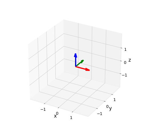
Fig. 2.7 Generic 3 axis Euclidean base. z axis obtained using hte cross product on x and y.¶

2.2.3. Matrices¶

Matrices $M_{n \times m}$ represents tables of numericals composed by $n$ rows and $m$ columns. Each component of the matrix $M_{i,j}$ can be referred by a row index $1 \leq i \leq n$ and column index $1 \leq j \leq m$. A matrix can also be seen as a container of $m$ column vectors of dimension $n$. We say $M$ is an $n$ by $m$ matrix and contains $m \times n$ elements. A Vector can be interpreted as a $n \times 1$, and a Scalar as a $1 \times 1$ Matrix.

\[\begin{split} M_{n \times m} = \begin{align} \begin{bmatrix} m_{1, 1} & m_{1, 2} & \dots & m_{1, m} \\ m_{2, 1} & m_{2, 2} & \dots & m_{2, m} \\ \vdots & \vdots & \ddots & \vdots \\ m_{n, 1} & m_{n, 2} & \dots & m_{n, m} \end{bmatrix} & = \begin{bmatrix} | & | & & | \\ \vec{v_1} & \vec{v_2} & \dots & \vec{v_m} \\ | & | & & | \end{bmatrix} \end{align} \end{split}\]

import numpy as np

# 2 by 3 matrix
data = np.array([
    # 1  2  3
    [1, 0, 0], # 1
    [0, 1, 0], # 2
])

data.shape, data.size

((2, 3), 6)

import numpy as np
import matplotlib.pyplot as plt
plt.ion()
plt.style.use('fivethirtyeight')

fig = plt.figure(figsize=(8, 4), facecolor="white")
ax1, ax2 = [fig.add_subplot(1, 2, i + 1) for i in range(2)]

img = ax1.imshow(data, interpolation="nearest", cmap="gray")
ax1.set_xticks(range(3))
ax1.set_yticks(range(2))
ax1.set_xticklabels([f"v_{i}" for i in range(1, 3 + 1)])
ax1.set_yticklabels(["x", "y"])
ax1.tick_params(axis=u"both", which=u"both", length=0)
ax1.grid(False)
ax1.title.set_text("Image Matrix")

ax2.scatter(data[0, :], data[1, :])
ax2.set_xlim(-1, 2)
ax2.set_ylim(-1, 2)
ax2.set_xticks(range(0, 2))
ax2.set_yticks(range(0, 2))
ax2.set_xlabel("x")
ax2.set_ylabel("y")
ax2.set_aspect("equal")
for i, (x, y) in enumerate(zip(data[0, :], data[1, :]), start=1):
    ax2.annotate(f"v_{i}", (x + .1, y + .1), fontsize=12)
ax2.title.set_text("Matrix' Vectors")

fig.subplots_adjust(hspace=0.25, wspace=0.40)
fig.canvas.draw()

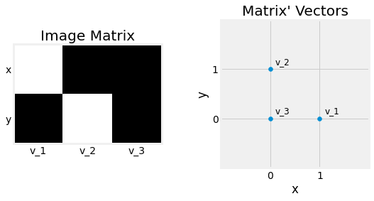
Fig. 2.8 Two visualisations of the matrix $\begin{bmatrix}1&0&0\\0&1&0\end{bmatrix}$ composed of the $3$ vectors $\begin{pmatrix}1\\0\end{pmatrix}$, $\begin{pmatrix}0\\1\end{pmatrix}$, and $\begin{pmatrix}0\\0\end{pmatrix}$, as an image left and as point coordinates right.¶

2.2.3.1. Scaling and Addition¶

As Vectors and Scalars, two Matrices of the same size can be added together. A Matrix can also be scaled by a Scalar.

\[\begin{split} \begin{align} A + B = \begin{bmatrix} | & | & & | \\ \vec{a_1} + \vec{b_1} & \vec{a_2} + \vec{b_2} & \dots & \vec{a_m} + \vec{b_m} \\ | & | & & | \end{bmatrix} && sA = \begin{bmatrix} | & | & & | \\ s\vec{a_1} & s\vec{a_2} & \dots & s\vec{a_m} \\ | & | & & | \end{bmatrix} \end{align} \end{split}\]

2.2.3.2. Transpose¶

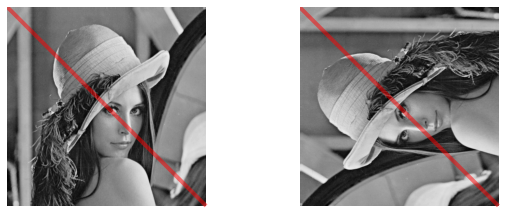
The Transpose of a matrix $M^T$ is obtained by flipping its rows and columns. The $n \times m$ Matrix becomes an $m \times n$ by transposition.

\[\begin{split} M^T = \begin{align} \begin{bmatrix} m_{1, 1} & m_{2, 1} & \dots & m_{n, 1} \\ m_{1, 2} & m_{2, 2} & \dots & m_{n, 2} \\ \vdots & \vdots & \ddots & \vdots \\ m_{1, m} & m_{2, m} & \dots & m_{n, m} \end{bmatrix} & = \begin{bmatrix} ─ & \vec{v_1}^T & ─ \\ ─ & \vec{v_2}^T & ─ \\ & \vdots & \\ ─ & \vec{v_m}^T & ─ \\ \end{bmatrix} \end{align} \end{split}\]

import numpy as np

M = np.array([
    [1, 0 , 0],
    [0, 1 , 0],
])

M_t = M.T

M_t, M_t.shape

(array([[1, 0],
        [0, 1],
        [0, 0]]),
 (3, 2))

from io import BytesIO
from PIL import Image

import numpy as np
import matplotlib.pyplot as plt
plt.ion()
plt.style.use('fivethirtyeight')

import requests

url = "https://upload.wikimedia.org/wikipedia/en/7/7d/Lenna_%28test_image%29.png"
response = requests.get(url)
img = np.array(Image.open(BytesIO(response.content)).convert("L"))

fig = plt.figure(figsize=(8, 4), facecolor="white")
ax1, ax2 = [fig.add_subplot(1, 2, i + 1) for i in range(2)]

ax1.imshow(img, cmap="gray")
ax1.plot([0, img.shape[1]], [0, img.shape[0]], color="r", alpha=0.5)
ax1.set_axis_off()

ax2.imshow(img.T, cmap="gray")
ax2.plot([0, img.shape[0]], [0, img.shape[1]], color="r", alpha=0.5)
ax2.set_axis_off()

fig.subplots_adjust(hspace=0.25, wspace=0.40)
fig.canvas.draw()

Fig. 2.9 Grayscale image of Lenna, a matrix of size $h \times w$ left, and its transpose of size $w \times h$ right.¶

2.2.3.3. Hadamard Product¶

The Hadamard product is an element-wise product and requires the two matrices to be of the same dimensionality.

\[\begin{split} A \odot B = \begin{bmatrix} a_{1, 1} b_{1, 1} & a_{1, 2} b_{1, 2} & \dots & a_{1, m} b_{1, m} \\ a_{2, 1} b_{2, 1} & a_{2, 2} b_{2, 2} & \dots & a_{2, m} b_{2, m} \\ \vdots & \vdots & \ddots & \vdots \\ a_{n, 1} b_{n, 1} & a_{n, 2} b_{n, 2} & \dots & a_{n, m} b_{n, m} \end{bmatrix} \end{split}\]

2.2.3.4. Matrix Multiplication¶

The Matrix multiplication (dot product) can be defined as a weighted sum of the column of the second matrix. The matrices need to follow a size constraint. We need to consider a matrix $A$ of size $n \times m$ and $B$ of size $m \times p$. The number of columns of the first matrix has to correspond to the number of rows of the second. The result produces a Matrix of size $n \times p$.

\[ AB_{i, j} = \sum_{k=1}^p a_{i, k} b_{k, j} \]

It may be easier to interpret the matrix multiplication as the sum of weighted column vectors. Here is a simple numerical example to demonstrate this fact:

\[\begin{split} \begin{equation} \begin{split} AB & = \begin{bmatrix}1 & 0 & 2 \\ 4 & 2 & 3\end{bmatrix} \begin{bmatrix}2 & 1 \\ 0 & 1 \\ 3 & 4 \end{bmatrix} = \begin{bmatrix} 8 & 9 \\ 17 & 18 \end{bmatrix} \\ & = \begin{pmatrix} 1 \\ 4 \end{pmatrix} \begin{pmatrix} 2 & 1 \end{pmatrix} + \begin{pmatrix} 0 \\ 2 \end{pmatrix} \begin{pmatrix} 0 & 1 \end{pmatrix} + \begin{pmatrix} 2 \\ 3 \end{pmatrix} \begin{pmatrix} 3 & 4 \end{pmatrix} \end{split} \end{equation} \end{split}\]

import numpy as np

A = np.array([
    [1, 0, 2],
    [4, 2, 3],
])

B = np.array([
    [2, 1],
    [0, 1],
    [3, 4],
])

A_hadammard_A = A * A
A_mul_B = A @ B

print(f"Hadammar product:\n{A_hadammard_A}\nshape:\n{A_hadammard_A.shape}\n")
print(f"Matrix Mumtiplication:\n{A_mul_B}\nshape:\n{A_mul_B.shape}")

Hadammar product:
[[ 1  0  4]
 [16  4  9]]
shape:
(2, 3)

Matrix Mumtiplication:
[[ 8  9]
 [17 18]]
shape:
(2, 2)

2.3. Square Matrices¶

Square Matrix contains as many rows as they have columns, $n \times n$. For short, we describe A as a square matrix of size $n$. Square matrices can be added and multiplied together.

2.3.1. Diagonal and Triangular Matrices¶

A matrix with every component set to zeros except its main diagonal numerals is called a Diagonal Matrix. If all components above the diagonal of a square matrix are zeros, it is called a Lower Triangular Matrix, respectively Upper Triangular Matrix if all components under the main diagonal are zeros.

\[\begin{split} \begin{align} D_n = \begin{bmatrix} d_{1, 1} & 0 & \dots & 0 \\ 0 & d_{2, 1} & \dots & 0 \\ \vdots & \vdots & \ddots & \vdots \\ 0 & 0 & \dots & d_{n, n} \end{bmatrix} && L_n = \begin{bmatrix} l_{1, 1} & 0 & \dots & 0 \\ l_{2, 1} & l_{2, 2} & \dots & 0 \\ \vdots & \vdots & \ddots & \vdots \\ l_{n, 1} & l_{n, 2} & \dots & l_{n, n} \end{bmatrix} && U_n = \begin{bmatrix} u_{1, 1} & u_{1, 2} & \dots & u_{1, n} \\ 0 & u_{2, 2} & \dots & u_{2, n} \\ \vdots & \vdots & \ddots & \vdots \\ 0 & 0 & \dots & u_{n, n} \end{bmatrix} \end{align} \end{split}\]

import numpy as np


I3 = np.eye(3)                  # Identity Matrix of size 3
L3 = np.tril(np.ones(3))        # Lower Triangular Matrix of size 3
U3 = 1 - np.tril(np.ones(3))    # Upper Triangular Matrix of size 3

import numpy as np
import matplotlib.pyplot as plt
plt.ion()
plt.style.use('fivethirtyeight')

fig = plt.figure(figsize=(12, 4), facecolor="white")
ax1, ax2, ax3 = [fig.add_subplot(1, 3, i + 1) for i in range(3)]

ax1.imshow(np.eye(16), interpolation="nearest", cmap="gray")
ax1.set_axis_off()
ax1.title.set_text("Diagonal")

ax2.imshow(np.tril(np.ones(16)), interpolation="nearest", cmap="gray")
ax2.set_axis_off()
ax2.title.set_text("Lower Triangular")

ax3.imshow(1 - np.tril(np.ones(16)), interpolation="nearest", cmap="gray")
ax3.set_axis_off()
ax3.title.set_text("Upper Triangular")

fig.subplots_adjust(hspace=0.25, wspace=0.40)
fig.canvas.draw()

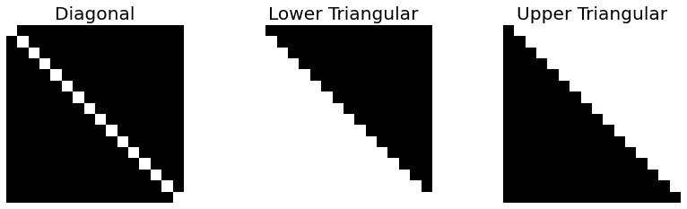
Fig. 2.10 $16 \times 16$ sqaures matrices, Diagonal, Lower Triangular, Upper Triangular. White is $1$, black is $0$.¶

2.3.2. Identity¶

We define the Identity Matrix $I_n$ as the diagonal matrix with its diagonal numericals set to one:

\[\begin{split} I_n = \begin{bmatrix} 1 & 0 & \dots & 0 \\ 0 & 1 & \dots & 0 \\ \vdots & \vdots & \ddots & \vdots \\ 0 & 0 & \dots & 1 \end{bmatrix} \end{split}\]

Its name is due to the fact that its matrix multiplication with any matrix returns the matrix unchanged: $A I_n = I_n A = A$

2.3.3. Special Square Matrices¶

A lot of Special Square Matrices exists and will not be stated in this chapter. Nevertheless, here is an example set of such matrices:

Symetric if $A=A^T$
Invetible if $A^{-1}$ existe tel que $AA^{-1}=A^{-1}A=I_n$
Normal if $A^T A = A A^T$
Orthogonal if $A^T=A^{-1}$

2.3.4. Trace¶

The Trace of a Matrix $tr(M)$ is the sum its diagonal components:

\[ \begin{align}tr(AB) = tr(BA) && tr(A) = tr(A^T)\end{align} \]

import numpy as np

#
#    (1, 0, 0)         (1, 1, 1)    
# tr (0, 1, 0) = 3  tr (1, 1, 1) = 3
#    (0, 0, 1)         (1, 1, 1)    
np.eye(3).trace(), np.ones((3, 3)).trace()

(3.0, 3.0)

2.3.5. Determinant¶

The Determinant of a sqaure matrix $det(M)$ encodes its properties. For example, a matrix is invertible if and only if its determinant is nonzero.

In 2D, the determinant is computed as follow:

\[\begin{split} \begin{vmatrix} a & b \\ c & d \end{vmatrix} = ad - bc \end{split}\]

In 3D, the determinant is computed as follow:

\[\begin{split} \begin{equation} \begin{split} \begin{vmatrix} a & b & c \\ d & e & f \\ g & h & i \end{vmatrix} & = a.\begin{vmatrix}e & f \\ h & i\end{vmatrix} - d.\begin{vmatrix}b & c \\ h & i\end{vmatrix} + g.\begin{vmatrix}b & c \\ e & f\end{vmatrix} \\ & = a(ei - hf) - d(bi - he) + g(bf - ec) \\ & = aei - ahf - dbi + dhc + gbf - gec \end{split} \end{equation} \end{split}\]

The computation of the determinant can be generalized to higher dimensions and defined in terms of permutations:

\[ det(M) = \sum_{\sigma \in \Sigma} (sgn(\sigma) \prod_{i=1}^n m_{i, \sigma_i}) \]

If we consider a Matrix as a set of basis vectors, the determinant represents the signed area in 2D, volume in 3D, …, of the n-dimensional parallelotope.

import numpy as np    
    
    
A = np.array([
    [0, 2],
    [1, 0],
])

det_A = np.linalg.det(A)
A_inv = np.linalg.inv(A) 

A @ A_inv, det_A

(array([[1., 0.],
        [0., 1.]]),
 -2.0)

import numpy as np
import matplotlib.pyplot as plt
import matplotlib.patches as plp
plt.ion()
plt.style.use('fivethirtyeight')

fig = plt.figure(figsize=(4, 4), facecolor="white")
ax = fig.add_subplot(1, 1, 1)

X = np.array([0, 0])
Y = np.array([0, 0])
U = np.array([1, 0])
V = np.array([0, 1])
C = ["r", 'g']

ax.quiver(X, Y, U, V, color=C, units='xy', scale=1)
ax.add_patch(plp.Rectangle([X[0], Y[0]], 1, 1, color="b", alpha=0.2))
ax.set_xlim(-1, 2)
ax.set_ylim(-1, 2)
ax.set_xticks(range(0, 1 + 1))
ax.set_yticks(range(0, 1 + 1))
ax.set_xlabel("x")
ax.set_ylabel("y")
ax.set_aspect("equal")

fig.subplots_adjust(hspace=0.25, wspace=0.40)
fig.canvas.draw()

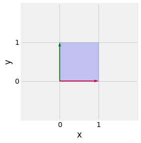
Fig. 2.11 Visualisation of the determinant of the $I_2$ matrix. $|I_2| = 1$ and the area of a unit square $1$.¶

2.4. Linear Transformations¶

Square matrices are pretty useful in the Computer Graphics domain as it can be used to represent all kinds of Spatial transformations $T$ needed to represent an object transform. Among those transformations are Linear Transformations: Scale, Rotation, Shearing, Reflection and Orthogonal Projection. They have to particularity to allow stacking those transformations using matrix multiplication (order dependant).

\[ \vec{u} = T \vec{v} \]

2.4.1. Scale¶

\[\begin{split} \begin{align} \begin{bmatrix} s_x & 0 \\ 0 & s_y \end{bmatrix} && \begin{bmatrix} s_x & 0 & 0 \\ 0 & s_y & 0 \\ 0 & 0 & s_z \\ \end{bmatrix} \end{align} \end{split}\]

from mpl_toolkits.mplot3d import Axes3D
from mpl_toolkits.mplot3d.art3d import Poly3DCollection, Line3DCollection

import numpy as np
import matplotlib.pyplot as plt
plt.ion()
plt.style.use('fivethirtyeight')


def cube_verts(cube: np.ndarray) -> np.ndarray:
    vectors = [*(cube[i] - cube[0] for i in range(1, 3 + 1))]
    verts = cube.tolist()
    verts += [cube[0] + vectors[0] + vectors[1]]
    verts += [cube[0] + vectors[0] + vectors[2]]
    verts += [cube[0] + vectors[1] + vectors[2]]
    verts += [cube[0] + vectors[0] + vectors[1] + vectors[2]]
    return np.array(verts).T
    
    
def cube_edges(verts: np.ndarray) -> np.ndarray:
    return np.array([
        [verts[0], verts[3], verts[5], verts[1]],
        [verts[1], verts[5], verts[7], verts[4]],
        [verts[4], verts[2], verts[6], verts[7]],
        [verts[2], verts[6], verts[3], verts[0]],
        [verts[0], verts[2], verts[4], verts[1]],
        [verts[3], verts[6], verts[7], verts[5]],
    ])


fig = plt.figure(figsize=(16, 8), facecolor="white")
ax1 = fig.add_subplot(1, 2, 1)
ax2 = fig.add_subplot(1, 2, 2, projection="3d")

X = np.array([
    [1, 0],
    [0, 1],
])

S = np.array([
    [2.0, 0.0],
    [0.0, 0.5],
])
SX = S @ X

ax1.scatter(X[0, :], X[1, :], s=100)
ax1.scatter(SX[0, :], SX[1, :], s=100)
ax1.set_xticks(range(0, 2 + 1))
ax1.set_yticks(range(0, 1 + 1))
ax1.set_xlim(-1, 3)
ax1.set_ylim(-1, 2)
ax1.set_xlabel("x")
ax1.set_ylabel("y")
ax1.set_aspect("equal")
ax1.title.set_text("2D")

X = cube_verts(np.array((
    (0, 0, 0),
    (0, 1, 0),
    (1, 0, 0),
    (0, 0, 1),
)))

S = np.array([
    [2.0, 0.0, 0.0],
    [0.0, 1.0, 0.0],
    [0.0, 0.0, 0.5],
])
SX = S @ X

cube1 = Poly3DCollection(cube_edges(X.T), linewidths=1, edgecolors='k')
cube1.set_facecolor((1, 0, 0, 0.1))
cube1.set_edgecolor((1, 0, 0, 1.0))

cube2 = Poly3DCollection(cube_edges(SX.T), linewidths=1, edgecolors='k')
cube2.set_facecolor((0, 0, 1, 0.1))
cube2.set_edgecolor((0, 0, 1, 1.0))

ax2.figure.gca(projection='3d')
ax2.add_collection3d(cube1)
ax2.add_collection3d(cube2)
ax2.set_xticks(np.arange(0, 1 + 1))
ax2.set_yticks(np.arange(0, 1 + 1))
ax2.set_zticks(np.arange(0, 1 + 1))
ax2.set_xlim(-1, 2)
ax2.set_ylim(-1, 2)
ax2.set_zlim(-1, 2)
ax2.set_xlabel("x")
ax2.set_ylabel("y")
ax2.set_zlabel("z")
ax2.patch.set_facecolor('white')
ax2.dist = 12
ax2.title.set_text("3D")

fig.canvas.draw()

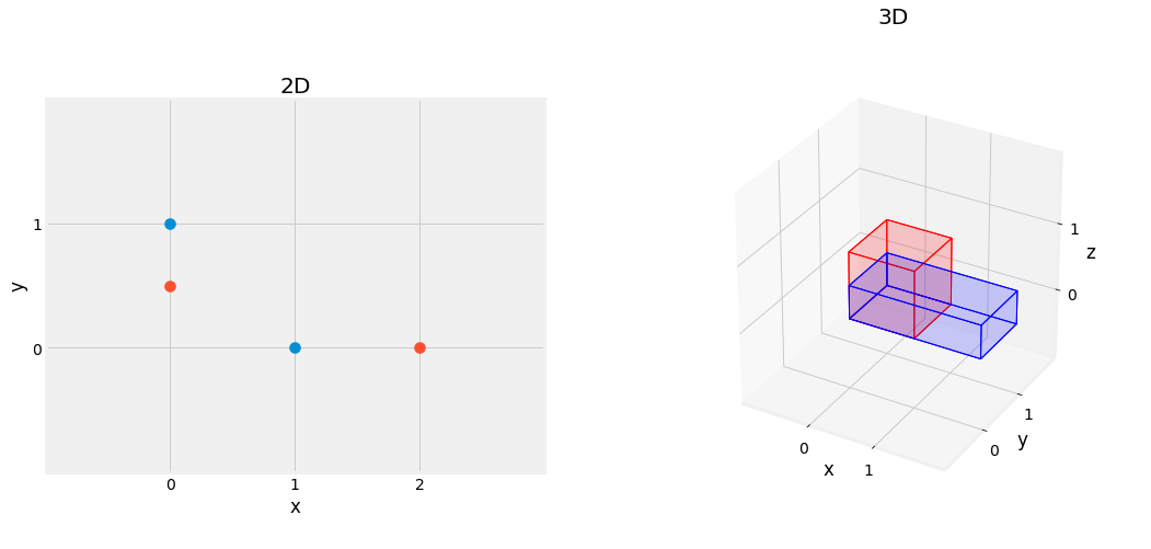
Fig. 2.12 Effect of Scaling Matrix, scaling by $2$ on x axis, $0.5$ on y axis, left figure, scaling by $2$ on x axis, $0.5$ on z axis, right figure.¶

2.4.2. Rotation¶

\[\begin{split} \begin{bmatrix} cos(\theta) & -sin(\theta) \\ sin(\theta) & cos(\theta) \end{bmatrix} \end{split}\]

\[\begin{split} \begin{align} \begin{bmatrix} 1 & 0 & 0 \\ 0 & cos(\theta) & -sin(\theta) \\ 0 & sin(\theta) & cos(\theta) \\ \end{bmatrix} && \begin{bmatrix} cos(\theta) & 0 & sin(\theta) \\ 0 & 1 & 0 \\ -sin(\theta) & 0 & cos(\theta) \\ \end{bmatrix} && \begin{bmatrix} cos(\theta) & -sin(\theta) & 0 \\ sin(\theta) & cos(\theta) & 0 \\ 0 & 0 & 1 \\ \end{bmatrix} \end{align} \end{split}\]

from mpl_toolkits.mplot3d import Axes3D
from mpl_toolkits.mplot3d.art3d import Poly3DCollection, Line3DCollection

import numpy as np
import matplotlib.pyplot as plt
plt.ion()
plt.style.use('fivethirtyeight')


def cube_verts(cube: np.ndarray) -> np.ndarray:
    vectors = [*(cube[i] - cube[0] for i in range(1, 3 + 1))]
    verts = cube.tolist()
    verts += [cube[0] + vectors[0] + vectors[1]]
    verts += [cube[0] + vectors[0] + vectors[2]]
    verts += [cube[0] + vectors[1] + vectors[2]]
    verts += [cube[0] + vectors[0] + vectors[1] + vectors[2]]
    return np.array(verts).T
    
    
def cube_edges(verts: np.ndarray) -> np.ndarray:
    return np.array([
        [verts[0], verts[3], verts[5], verts[1]],
        [verts[1], verts[5], verts[7], verts[4]],
        [verts[4], verts[2], verts[6], verts[7]],
        [verts[2], verts[6], verts[3], verts[0]],
        [verts[0], verts[2], verts[4], verts[1]],
        [verts[3], verts[6], verts[7], verts[5]],
    ])


fig = plt.figure(figsize=(16, 8), facecolor="white")
ax1 = fig.add_subplot(1, 2, 1)
ax2 = fig.add_subplot(1, 2, 2, projection="3d")

theta = 45 * np.pi / 180
X = np.array([
    [1, 0],
    [0, 1],
])

R = np.array([
    [np.cos(theta), -np.sin(theta)],
    [np.sin(theta),  np.cos(theta)],
])
RX = R @ X

ax1.scatter(X[0, :], X[1, :], s=100)
ax1.scatter(RX[0, :], RX[1, :], s=100)
ax1.set_xticks(range(-1, 1 + 1))
ax1.set_yticks(range(0, 1 + 1))
ax1.set_xlim(-2, 2)
ax1.set_ylim(-1, 2)
ax1.set_xlabel("x")
ax1.set_ylabel("y")
ax1.set_aspect("equal")
ax1.title.set_text("2D")

X = cube_verts(np.array((
    (0, 0, 0),
    (0, 1, 0),
    (1, 0, 0),
    (0, 0, 1),
)))

theta = 45 * np.pi / 180
Rx = np.array([
    [1.0,           0.0,            0.0],
    [0.0, np.cos(theta), -np.sin(theta)],
    [0.0, np.sin(theta),  np.cos(theta)],
])
RxX = Rx @ X

Rz = np.array([
    [np.cos(theta), -np.sin(theta), 0.0],
    [np.sin(theta),  np.cos(theta), 0.0],
    [          0.0,            0.0, 1.0],
])
RzX = Rz @ X

cube1 = Poly3DCollection(cube_edges(X.T), linewidths=1, edgecolors='k')
cube1.set_facecolor((1, 0, 0, 0.1))
cube1.set_edgecolor((1, 0, 0, 1.0))

cube2 = Poly3DCollection(cube_edges(RxX.T), linewidths=1, edgecolors='k')
cube2.set_facecolor((0, 0, 1, 0.1))
cube2.set_edgecolor((0, 0, 1, 1.0))

cube3 = Poly3DCollection(cube_edges(RzX.T), linewidths=1, edgecolors='k')
cube3.set_facecolor((0, 1, 0, 0.1))
cube3.set_edgecolor((0, 1, 0, 1.0))

ax2.figure.gca(projection='3d')
ax2.add_collection3d(cube1)
ax2.add_collection3d(cube2)
ax2.add_collection3d(cube3)
ax2.set_xticks(np.arange(0, 1 + 1))
ax2.set_yticks(np.arange(0, 1 + 1))
ax2.set_zticks(np.arange(0, 1 + 1))
ax2.set_xlim(-1, 2)
ax2.set_ylim(-1, 2)
ax2.set_zlim(-1, 2)
ax2.set_xlabel("x")
ax2.set_ylabel("y")
ax2.set_zlabel("z")
ax2.patch.set_facecolor('white')
ax2.dist = 12
ax2.title.set_text("3D")

fig.canvas.draw()

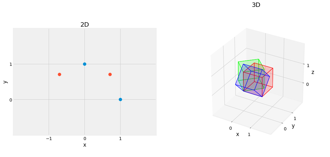
Fig. 2.13 Effect of Rotation Matrix, rotating the figure by $45^{\circ}$ left figure, and $45^{\circ}$ on the $x$ axis in blue, and on the $z$ axis in green, right figure.¶

2.4.3. Shearing¶

\[\begin{split} \begin{align} \begin{bmatrix} 1 & \lambda \\ 0 & 1 \end{bmatrix} && \begin{bmatrix} 1 & \lambda_{xy} & \lambda_{xz} \\ \lambda_{yx} & 1 & \lambda_{yz} \\ \lambda_{zx} & \lambda_{zy} & 1 \\ \end{bmatrix} \end{align} \end{split}\]

from mpl_toolkits.mplot3d import Axes3D
from mpl_toolkits.mplot3d.art3d import Poly3DCollection, Line3DCollection

import numpy as np
import matplotlib.pyplot as plt
plt.ion()
plt.style.use('fivethirtyeight')


def cube_verts(cube: np.ndarray) -> np.ndarray:
    vectors = [*(cube[i] - cube[0] for i in range(1, 3 + 1))]
    verts = cube.tolist()
    verts += [cube[0] + vectors[0] + vectors[1]]
    verts += [cube[0] + vectors[0] + vectors[2]]
    verts += [cube[0] + vectors[1] + vectors[2]]
    verts += [cube[0] + vectors[0] + vectors[1] + vectors[2]]
    return np.array(verts).T
    
    
def cube_edges(verts: np.ndarray) -> np.ndarray:
    return np.array([
        [verts[0], verts[3], verts[5], verts[1]],
        [verts[1], verts[5], verts[7], verts[4]],
        [verts[4], verts[2], verts[6], verts[7]],
        [verts[2], verts[6], verts[3], verts[0]],
        [verts[0], verts[2], verts[4], verts[1]],
        [verts[3], verts[6], verts[7], verts[5]],
    ])


fig = plt.figure(figsize=(16, 8), facecolor="white")
ax1 = fig.add_subplot(1, 2, 1)
ax2 = fig.add_subplot(1, 2, 2, projection="3d")

theta = 45 * np.pi / 180
X = np.array([
    [1, 1, 0, 0],
    [1, 0, 1, 0],
])

Sh = np.eye(2)
Sh[0, 1] = -1.0
ShX = Sh @ X

ax1.scatter(X[0, :], X[1, :], s=100, alpha=0.5)
ax1.scatter(ShX[0, :], ShX[1, :], s=100, alpha=0.5)
ax1.set_xticks(range(-1, 1 + 1))
ax1.set_yticks(range(0, 1 + 1))
ax1.set_xlim(-2, 2)
ax1.set_ylim(-1, 2)
ax1.set_xlabel("x")
ax1.set_ylabel("y")
ax1.set_aspect("equal")
ax1.title.set_text("2D")

X = cube_verts(np.array((
    (0, 0, 0),
    (0, 1, 0),
    (1, 0, 0),
    (0, 0, 1),
)))

Sh = np.eye(3)
Sh[0, 2] = -1.0
ShX = Sh @ X

cube1 = Poly3DCollection(cube_edges(X.T), linewidths=1, edgecolors='k')
cube1.set_facecolor((1, 0, 0, 0.1))
cube1.set_edgecolor((1, 0, 0, 1.0))

cube2 = Poly3DCollection(cube_edges(ShX.T), linewidths=1, edgecolors='k')
cube2.set_facecolor((0, 0, 1, 0.1))
cube2.set_edgecolor((0, 0, 1, 1.0))

ax2.figure.gca(projection='3d')
ax2.add_collection3d(cube1)
ax2.add_collection3d(cube2)
ax2.set_xticks(np.arange(0, 1 + 1))
ax2.set_yticks(np.arange(0, 1 + 1))
ax2.set_zticks(np.arange(0, 1 + 1))
ax2.set_xlim(-1, 2)
ax2.set_ylim(-1, 2)
ax2.set_zlim(-1, 2)
ax2.set_xlabel("x")
ax2.set_ylabel("y")
ax2.set_zlabel("z")
ax2.patch.set_facecolor('white')
ax2.dist = 12
ax2.title.set_text("3D")

fig.canvas.draw()

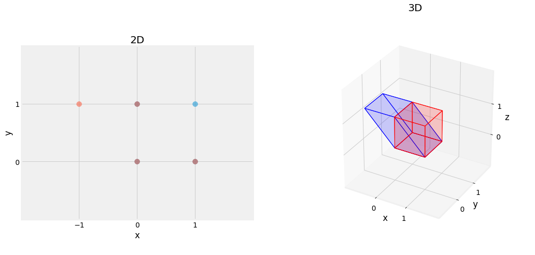
Fig. 2.14 Effect of Shearing Matrix, shearing figure on the $x$-axis.¶

2.4.4. Reflection¶

\[\begin{split} \begin{align} \begin{bmatrix} \delta_x & 0 \\ 0 & \delta_y \end{bmatrix} && \begin{bmatrix} \delta_x & 0 & 0 \\ 0 & \delta_y & 0 \\ 0 & 0 & \delta_z \\ \end{bmatrix} && \delta \in \{-1; 1\} \end{align} \end{split}\]

from mpl_toolkits.mplot3d import Axes3D
from mpl_toolkits.mplot3d.art3d import Poly3DCollection, Line3DCollection

import numpy as np
import matplotlib.pyplot as plt
plt.ion()
plt.style.use('fivethirtyeight')


def cube_verts(cube: np.ndarray) -> np.ndarray:
    vectors = [*(cube[i] - cube[0] for i in range(1, 3 + 1))]
    verts = cube.tolist()
    verts += [cube[0] + vectors[0] + vectors[1]]
    verts += [cube[0] + vectors[0] + vectors[2]]
    verts += [cube[0] + vectors[1] + vectors[2]]
    verts += [cube[0] + vectors[0] + vectors[1] + vectors[2]]
    return np.array(verts).T
    
    
def cube_edges(verts: np.ndarray) -> np.ndarray:
    return np.array([
        [verts[0], verts[3], verts[5], verts[1]],
        [verts[1], verts[5], verts[7], verts[4]],
        [verts[4], verts[2], verts[6], verts[7]],
        [verts[2], verts[6], verts[3], verts[0]],
        [verts[0], verts[2], verts[4], verts[1]],
        [verts[3], verts[6], verts[7], verts[5]],
    ])


fig = plt.figure(figsize=(16, 8), facecolor="white")
ax1 = fig.add_subplot(1, 2, 1)
ax2 = fig.add_subplot(1, 2, 2, projection="3d")

theta = 45 * np.pi / 180
X = np.array([
    [1, 1, 0, 0],
    [1, 0, 1, 0],
])

Rf = -np.eye(2)
RfX = Rf @ X

ax1.scatter(X[0, :], X[1, :], s=100, alpha=0.5)
ax1.scatter(RfX[0, :], RfX[1, :], s=100, alpha=0.5)
ax1.set_xticks(range(-1, 1 + 1))
ax1.set_yticks(range(-1, 1 + 1))
ax1.set_xlim(-2, 2)
ax1.set_ylim(-2, 2)
ax1.set_xlabel("x")
ax1.set_ylabel("y")
ax1.set_aspect("equal")
ax1.title.set_text("2D")

X = cube_verts(np.array((
    (0, 0, 0),
    (0, 1, 0),
    (1, 0, 0),
    (0, 0, 1),
)))

Rf = -np.eye(3)
RfX = Rf @ X

cube1 = Poly3DCollection(cube_edges(X.T), linewidths=1, edgecolors='k')
cube1.set_facecolor((1, 0, 0, 0.1))
cube1.set_edgecolor((1, 0, 0, 1.0))

cube2 = Poly3DCollection(cube_edges(RfX.T), linewidths=1, edgecolors='k')
cube2.set_facecolor((0, 0, 1, 0.1))
cube2.set_edgecolor((0, 0, 1, 1.0))

ax2.figure.gca(projection='3d')
ax2.add_collection3d(cube1)
ax2.add_collection3d(cube2)
ax2.set_xticks(np.arange(-1, 1 + 1))
ax2.set_yticks(np.arange(-1, 1 + 1))
ax2.set_zticks(np.arange(-1, 1 + 1))
ax2.set_xlim(-2, 2)
ax2.set_ylim(-2, 2)
ax2.set_zlim(-2, 2)
ax2.set_xlabel("x")
ax2.set_ylabel("y")
ax2.set_zlabel("z")
ax2.patch.set_facecolor('white')
ax2.dist = 12
ax2.title.set_text("3D")

fig.canvas.draw()

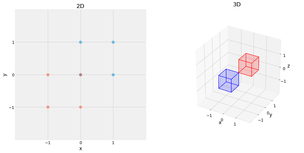
Fig. 2.15 Effect of Reflection Matrix, reflected on all axis (x and y left, x, y, and z right) in blue.¶

2.5. Affine Transformations¶

Some transformation matrices are able to preserve lines and parallelism. Those matrices are called Affine Transformation Matrices.

Affine Transformations are represented as a Linear Tranfromation $A$ followed by the addition of a one vector $\vec{b}$:

\[ \vec{y} = A \vec{x} + \vec{b} \]

This suit of matrix/vector operations is often simplified by a single matrix we call the Augmented Matrix.

\[\begin{split} \begin{bmatrix} \vec{y} \\ 1 \end{bmatrix} = \begin{bmatrix} A & \vec{b} \\ 0 & 1 \end{bmatrix} \begin{bmatrix} \vec{x} \\ 1 \end{bmatrix} \end{split}\]

2.5.1. Tranlsation¶

In the case of a Translation, $A$ is $I_n$, and $\vec{b}$ represents the translation respectively on each axis it is defined on.

from mpl_toolkits.mplot3d import Axes3D
from mpl_toolkits.mplot3d.art3d import Poly3DCollection, Line3DCollection

import numpy as np
import matplotlib.pyplot as plt
plt.ion()
plt.style.use('fivethirtyeight')


def cube_verts(cube: np.ndarray) -> np.ndarray:
    vectors = [*(cube[i] - cube[0] for i in range(1, 3 + 1))]
    verts = cube.tolist()
    verts += [cube[0] + vectors[0] + vectors[1]]
    verts += [cube[0] + vectors[0] + vectors[2]]
    verts += [cube[0] + vectors[1] + vectors[2]]
    verts += [cube[0] + vectors[0] + vectors[1] + vectors[2]]
    return np.array(verts).T
    
    
def cube_edges(verts: np.ndarray) -> np.ndarray:
    return np.array([
        [verts[0], verts[3], verts[5], verts[1]],
        [verts[1], verts[5], verts[7], verts[4]],
        [verts[4], verts[2], verts[6], verts[7]],
        [verts[2], verts[6], verts[3], verts[0]],
        [verts[0], verts[2], verts[4], verts[1]],
        [verts[3], verts[6], verts[7], verts[5]],
    ])


fig = plt.figure(figsize=(16, 8), facecolor="white")
ax1 = fig.add_subplot(1, 2, 1)
ax2 = fig.add_subplot(1, 2, 2, projection="3d")

theta = 45 * np.pi / 180
X = np.array([
    [1, 1, 0, 0],
    [1, 0, 1, 0],
    [1, 1, 1, 1],
])

T = np.eye(3)
T[0, 2] = -0.5
T[1, 2] = -0.5
TX = T @ X

ax1.scatter(X[0, :], X[1, :], s=100, alpha=0.5)
ax1.scatter(TX[0, :], TX[1, :], s=100, alpha=0.5)
ax1.set_xticks(range(-1, 1 + 1))
ax1.set_yticks(range(-1, 1 + 1))
ax1.set_xlim(-2, 2)
ax1.set_ylim(-2, 2)
ax1.set_xlabel("x")
ax1.set_ylabel("y")
ax1.set_aspect("equal")
ax1.title.set_text("2D")

V = cube_verts(np.array((
    (0, 0, 0),
    (0, 1, 0),
    (1, 0, 0),
    (0, 0, 1),
)))
X = np.vstack([V, np.ones((1, V.shape[1]))])

T = np.eye(4)
T[1, 3] = -1
TX1 = T @ X

T = np.eye(4)
T[0, 3] = -1
TX2 = T @ X

T = np.eye(4)
T[2, 3] = -1.0
TX3 = T @ X

cube1 = Poly3DCollection(cube_edges(X[:3].T), linewidths=1, edgecolors='k')
cube1.set_facecolor((1, 0, 0, 0.1))
cube1.set_edgecolor((1, 0, 0, 1.0))

cube2 = Poly3DCollection(cube_edges(TX1[:3].T), linewidths=1, edgecolors='k')
cube2.set_facecolor((0, 0, 1, 0.1))
cube2.set_edgecolor((0, 0, 1, 1.0))

cube3 = Poly3DCollection(cube_edges(TX2[:3].T), linewidths=1, edgecolors='k')
cube3.set_facecolor((0, 1, 0, 0.1))
cube3.set_edgecolor((0, 1, 0, 1.0))

cube4 = Poly3DCollection(cube_edges(TX3[:3].T), linewidths=1, edgecolors='k')
cube4.set_facecolor((1, 1, 0, 0.1))
cube4.set_edgecolor((1, 1, 0, 1.0))

ax2.figure.gca(projection='3d')
ax2.add_collection3d(cube1)
ax2.add_collection3d(cube2)
ax2.add_collection3d(cube3)
ax2.add_collection3d(cube4)
ax2.set_xticks(np.arange(-1, 1 + 1))
ax2.set_yticks(np.arange(-1, 1 + 1))
ax2.set_zticks(np.arange(-1, 1 + 1))
ax2.set_xlim(-2, 2)
ax2.set_ylim(-2, 2)
ax2.set_zlim(-2, 2)
ax2.set_xlabel("x")
ax2.set_ylabel("y")
ax2.set_zlabel("z")
ax2.patch.set_facecolor('white')
ax2.dist = 12
ax2.title.set_text("3D")

fig.canvas.draw()

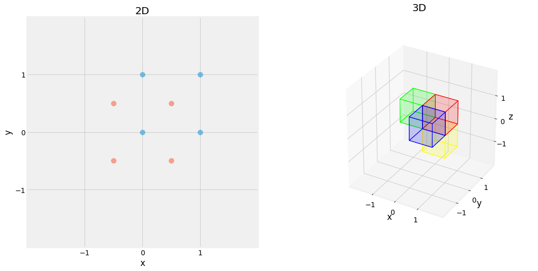
Fig. 2.16 Effect of Translation Matrix. Red square is translated by $\begin{pmatrix} -0.5 \\ -0.5 \end{pmatrix}$ in blue on left, and red cube is translated by $\begin{pmatrix} 0 \\ -1 \\ 0 \end{pmatrix}$ in blue, $\begin{pmatrix} -1 \\ 0 \\ 0 \end{pmatrix}$ in green, and $\begin{pmatrix} 0 \\ 0 \\ -1 \end{pmatrix}$ in yellow, on right.¶

2.6. Eigenvectors and Diagonalization¶

Eigenvectors are the essence of Linear Algebra.

2.6.1. Eigenvector¶

A Vector $\vec{x}$ is said to be an Eigenvector of the matrix $A$ when the following equation can be satisfied by a scalar $\lambda$ then called an Eigenvalue:

\[ A\vec{x} = \lambda \vec{x} \]

Eigenvectors for matrix $A$ represent vectors, which do not change in terms of its span when the transformation $A$ is applied. The eigenvalues $\lambda$ represents the strength of stretch given by $A$ for its corresponding eigenvector. An n-dimensional has a maximum of n eigenvalues and independent eigenvectors.

This definition gives us a direct way to compute eigenvalues as it can be rewritten in the following way:

\[\begin{split} \begin{equation} \begin{split} A\vec{x} - \lambda I \vec{x} & = 0 \\ (A - \lambda I) \vec{x} & = 0 \\ det(A - \lambda I) & = 0 \end{split} \end{equation} \end{split}\]

Any $\lambda \in \mathbb{R}$ that satisfies this equation is an eigenvalue.

The following method shows how to compute the eigenvectors and values of a $2 \times 2$ matrix but can be extended to any n square matrix. Let us consider the following matrix:

\[\begin{split} A = \begin{bmatrix} 3 & 1 \\ 1 & 3 \end{bmatrix} \end{split}\]

Step 1: Find the roots of the characteristic polynomial of $A$

\[\begin{split} \begin{equation} \begin{split} det(A - \lambda I_2) & = 0 \\ (3 - \lambda)^2 - 1 & = 0 \\ (2 - \lambda)(4 - \lambda) & = 0 \end{split} \end{equation} \end{split}\]

In this case we found out $\lambda_1 = 4$ and $\lambda_2 = 2$ are eigenvalues of the matrix $A$.

Step2: Replace $\lambda$ by the eigenvalue found and solve for $\vec{x}$

Replacing $\lambda$ by $\lambda_1 = 4$:

\[\begin{split} \begin{bmatrix} -1 & 1 \\ 1 & -1 \end{bmatrix} \vec{x_1} = 0 \end{split}\]

The vector $\vec{x_1}=\begin{pmatrix} 1 \\ 1 \end{pmatrix}$ satisfies the equation and can be assigned as one eigenvector for $A$ with eigenvalue $\lambda_1$.

Replacing $\lambda$ by $\lambda_2 = 2$:

\[\begin{split} \begin{bmatrix} 1 & 1 \\ 1 & 1 \end{bmatrix} \vec{x_2} = 0 \end{split}\]

The vector $\vec{x_2}=\begin{pmatrix} -1 \\ 1 \end{pmatrix}$ satisfies the equation and can be assigned as one eigenvector for $A$ with eigenvalue $\lambda_2$.

import numpy as np


A = np.array([
    [3, 1],
    [1, 3],
])

lambdas, eigen_vects = np.linalg.eig(A)
print(f"eigen value lambda_1: {lambdas[0]} w/ eigen vector x_1: {eigen_vects[:, 0]}")
print(f"eigen value lambda_2: {lambdas[1]} w/ eigen vector x_2: {eigen_vects[:, 1]}")

eigen value lambda_1: 4.0 w/ eigen vector x_1: [0.70710678 0.70710678]
eigen value lambda_2: 2.0 w/ eigen vector x_2: [-0.70710678  0.70710678]

from io import BytesIO
from matplotlib.ticker import MultipleLocator
from PIL import Image

import numpy as np
import matplotlib.pyplot as plt
plt.ion()
plt.style.use('fivethirtyeight')

import requests

url = "https://upload.wikimedia.org/wikipedia/en/7/7d/Lenna_%28test_image%29.png"
response = requests.get(url)
img1 = np.array(Image.open(BytesIO(response.content)).convert("L"))
img2 = np.array(Image.open(BytesIO(response.content)).convert("L").resize((256, 128)))

fig = plt.figure(figsize=(8, 4), facecolor="white")
ax1, ax2 = [fig.add_subplot(1, 2, i + 1) for i in range(2)]

X = np.array([ 0,  0])
Y = np.array([ 0,  0])
U = np.array([64,  0])
V = np.array([ 0, 64])
C = ["r", "g"]

img = ax1.imshow(img1, cmap="gray", alpha=0.6, extent=(-128, 128, -128, 128))
ax1.quiver(X, Y, U, V, color=C, units='xy', scale=1, linewidths=100)
ax1.set_xlabel("x")
ax1.set_ylabel("y")
plt.setp(ax1.get_xticklabels(), visible=False)
plt.setp(ax1.get_yticklabels(), visible=False)
ax1.tick_params(axis='both', which='both', length=0)
ax1.set_xlim(-256, 256)
ax1.set_ylim(-128, 128)
ax1.xaxis.set_major_locator(MultipleLocator(64))
ax1.yaxis.set_major_locator(MultipleLocator(64))
ax1.title.set_text("Before Transformation")

img = ax2.imshow(img2, cmap="gray", alpha=0.6, extent=(-256, 256, -128, 128))
ax2.quiver(X, Y, U * 2, V, color=C, units='xy', scale=1, linewidths=100)
ax2.set_xlabel("x")
ax2.set_ylabel("y")
plt.setp(ax2.get_xticklabels(), visible=False)
plt.setp(ax2.get_yticklabels(), visible=False)
ax2.tick_params(axis='both', which='both', length=0)
ax2.set_xlim(-256, 256)
ax2.set_ylim(-128, 128)
ax2.xaxis.set_major_locator(MultipleLocator(128))
ax2.yaxis.set_major_locator(MultipleLocator(64))
ax1.title.set_text("After Transformation")

fig.canvas.draw()

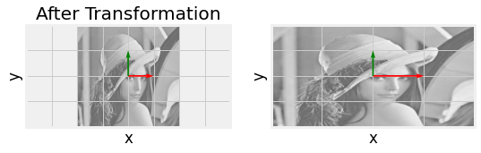
Fig. 2.17 Eigenvector visulaization for $\begin{bmatrix} 2 & 0 \\ 0 & 1 \end{bmatrix}$ with eigenvalues and vectors respectively $\begin{pmatrix} 0 \\ 1 \end{pmatrix}$, and $2 \begin{pmatrix} 1 \\ 0 \end{pmatrix}$. Notice how each eigenvector does not deviate from its span.¶

2.6.2. Diagonalisation¶

An n-dimensional matrix with a set of n normalized linearly independent eigenvectors can be Diagonalized in the following form with $V$ the matrix of n column eigenvectors and $\Lambda$ the diagonal matrix with the corresponding eigenvalues:

\[ A = V \Lambda V^{-1} \]

$V$ is called the left eigenvector, and $V^{-1}$ is the right eigenvector. If this affirmation does not convince you, one trivial example is the following:

\[\begin{split} A = \begin{bmatrix} a & 0 \\ 0 & b \end{bmatrix} = \begin{bmatrix} 1 & 0 \\ 0 & 1 \end{bmatrix} \begin{bmatrix} a & 0 \\ 0 & b \end{bmatrix} \begin{bmatrix} 1 & 0 \\ 0 & 1 \end{bmatrix} = I_2 A I_2^{-1} \end{split}\]

This matrix decomposition comes pretty handy in various situation du to its properties. For example, considering $f$ as any polynomial function:

\[ f(A) = V f(\Lambda) V^{-1} \]

import numpy as np


A = np.array([
    [3.0,  0.0],
    [1.0, -2.0],
])

lambdas, eigen_vectors = np.linalg.eig(A)

L = np.diag(lambdas)
V = eigen_vectors / eigen_vectors.max(axis=0)
V_1 = np.linalg.inv(V)

V @ L @ V_1

array([[ 3.,  0.],
       [ 1., -2.]])

2.7. Singular Value Decomposition¶

The Singular Value Decomposition, or SVD for short, is the Holy Grail of the modern Linear Algebra and is not limited to square matrices. The SVD consist of obtaining 3 matrices, the Left Singular Vectors $U$ of size $m \times m$, the Right Singular Vector $V$ of size $n \times n$ both orthonormal and $\Sigma$ a diagonal matrix of size $m \times n$ containing numerals called Singular Values.

\[\begin{split} \begin{equation} \begin{split} A & = USV^T \\ & = \begin{bmatrix} | & & | & & | \\ | & & | & & | \\ \vec{u_1} & \dots & \vec{u_n} & \dots & \vec{u_m} \\ | & & | & & | \\ | & & | & & | \\ \end{bmatrix} \begin{bmatrix} \sigma_1 & \dots & 0 \\ \vdots & \ddots & \vdots \\ 0 & \dots & \sigma_n \\ 0 & \dots & 0 \\ 0 & \ddots & 0 \\ 0 & \dots & 0 \\ \end{bmatrix} \begin{bmatrix} ─ & \vec{v_1}^T & ─ \\ & \dots & \\ ─ & \vec{v_n}^T & ─ \\ \end{bmatrix} \end{split} \end{equation} \end{split}\]

Note

The SVD does not require to compute the full left singular vectors and singular values. It can be simplified by ditching the null singular values, and their corresponding left and right singular vectors. This also saves memory and computation. This simplified version of the SVD is referred to as the economy SVD:

\[ A = \hat{U} \hat{\Sigma} \hat{V}^T \]

The SVD of a transformation matrix A tries to capture its essence as a Rotation and a Stretch. Its computation procedure is coming quite easily by computing the $AA^T$ and $A^TA$ matrices to solve for $U$ and $V$ separately.

\[\begin{split} \begin{equation} \begin{split} AA^T & = USV^TVS^TU^T \\ & = US^2U^T \end{split} \end{equation} \end{split}\]

\[\begin{split} \begin{equation} \begin{split} A^TA & = VS^TU^TUSV^T \\ & = VS^2V^T \end{split} \end{equation} \end{split}\]

Then, it is a matter of computing the orthonormal eigenvectors and values for the two matrices.

import numpy as np


A = np.array([
    [3, 2,  2],
    [2, 3, -2],
])

U, S, V_T = np.linalg.svd(A, full_matrices=False)

U @ np.diag(S) @ V_T

array([[ 3.,  2.,  2.],
       [ 2.,  3., -2.]])

More practically, the SVD of a transform matrix can be seen as a rotation (and/or reflection) $V^T$, a stretch $\Sigma$, and another rotation $U$. This decomposition has a real physical meaning and is relatively easy to interpret.

The SVD has the particularity to preserve unitary transformation matrices. Let us observe this phenomenon with an example:

import numpy as np


theta = np.array([12 * np.pi / 180, -340 * np.pi / 180, -350 * np.pi / 180])
Sigma = np.diag([2, 1, 0.5])

Rx = np.array([
    [1,                0,                 0],
    [0, np.cos(theta[0]), -np.sin(theta[0])],
    [0, np.sin(theta[0]),  np.cos(theta[0])],
])

Ry = np.array([
    [ np.cos(theta[0]), 0, np.sin(theta[0])],
    [               0,  1,                0],
    [-np.sin(theta[0]), 0, np.cos(theta[0])],
])

Rz = np.array([
    [np.cos(theta[0]), -np.sin(theta[0]), 0],
    [np.sin(theta[0]),  np.cos(theta[0]), 0],
    [               0,                 0, 1],
])

R = Rz @ Ry @ Rx
A = R @ Sigma
U, S, _ = np.linalg.svd(A, full_matrices=False)

print(f"A:\n{A}\n")
print(f"A (SVD):\n{U @ np.diag(S)}")

A:
[[ 1.91354546 -0.16108567  0.12107575]
 [ 0.40673664  0.96576018 -0.08054283]
 [-0.41582338  0.20336832  0.47838636]]

A (SVD):
[[-1.91354546  0.16108567  0.12107575]
 [-0.40673664 -0.96576018 -0.08054283]
 [ 0.41582338 -0.20336832  0.47838636]]

from mpl_toolkits.mplot3d import Axes3D
from typing import Tuple

import numpy as np
import matplotlib.pyplot as plt
plt.ion()
plt.style.use('fivethirtyeight')


array = np.ndarray
array3 = Tuple[array, array, array]
def apply_transformation(X: array, Y: array, Z: array, *, A: array) -> array3:
    M = A @ np.hstack([X.reshape(-1, 1), Y.reshape(-1, 1), Z.reshape(-1, 1)]).T
    return (
        M.T[:, 0].reshape(X.shape),
        M.T[:, 1].reshape(Y.shape),
        M.T[:, 2].reshape(Z.shape),
    )


def plot_axes(ax: plt.Figure, A: np.ndarray = np.eye(3)) -> None:
    M = A @ np.array([
        #x, y, z, u, v, w
        [0, 0, 0, 1, 0, 0],
        [0, 0, 0, 0, 1, 0],
        [0, 0, 0, 0, 0, 1],
    ])
    X, Y, Z, U, V, W = [M[:, i] for i in range(6)]
    for i, c in enumerate(["r", "g", "b"]):
        ax.quiver(
            X[i], Y[i], Z[i], U[i], V[i], W[i],
            color=c, length=2, arrow_length_ratio=0.2, linewidths=4,
        )
        
        
def plot_unit_sphere(ax: plt.Figure, A: np.ndarray = np.eye(3)) -> None:
    u = np.linspace(-np.pi, np.pi, 25)
    v = np.linspace(0, np.pi, 25)
    X = np.outer(np.cos(u), np.sin(v))
    Y = np.outer(np.sin(u), np.sin(v))
    Z = np.outer(np.ones_like(u), np.cos(v))
    X, Y, Z = apply_transformation(X, Y, Z, A=A)
    ax.plot_surface(X, Y, Z, color="b", alpha=0.1, shade=False, linewidth=0)


fig = plt.figure(figsize=(24, 8), facecolor="white")
ax1 = fig.add_subplot(1, 3, 1, projection="3d")
ax2 = fig.add_subplot(1, 3, 2, projection="3d")
ax3 = fig.add_subplot(1, 3, 3, projection="3d")

plot_unit_sphere(ax1)
plot_axes(ax1)
ax1.set_xlabel("x")
ax1.set_ylabel("y")
ax1.set_zlabel("z")
ax1.set_xlim(-2, 2)
ax1.set_ylim(-2, 2)
ax1.set_zlim(-2, 2)
ax1.set_xticks(range(-1, 2))
ax1.set_yticks(range(-1, 2))
ax1.set_zticks(range(-1, 2))
ax1.patch.set_facecolor('white')
ax1.dist = 12
ax1.title.set_text("Original")

plot_unit_sphere(ax2, A=A)
plot_axes(ax2, A=A)
ax2.set_xlabel("x")
ax2.set_ylabel("y")
ax2.set_zlabel("z")
ax2.set_xlim(-2, 2)
ax2.set_ylim(-2, 2)
ax2.set_zlim(-2, 2)
ax2.set_xticks(range(-1, 2))
ax2.set_yticks(range(-1, 2))
ax2.set_zticks(range(-1, 2))
ax2.patch.set_facecolor('white')
ax2.dist = 12
ax2.title.set_text("Transformed")

plot_unit_sphere(ax3, A=U @ np.diag(S))
plot_axes(ax3, A=U @ np.diag(S))
ax3.set_xlabel("x")
ax3.set_ylabel("y")
ax3.set_zlabel("z")
ax3.set_xlim(-2, 2)
ax3.set_ylim(-2, 2)
ax3.set_zlim(-2, 2)
ax3.set_xticks(range(-1, 2))
ax3.set_yticks(range(-1, 2))
ax3.set_zticks(range(-1, 2))
ax3.patch.set_facecolor('white')
ax3.dist = 12
ax3.title.set_text("SVD")

fig.canvas.draw()

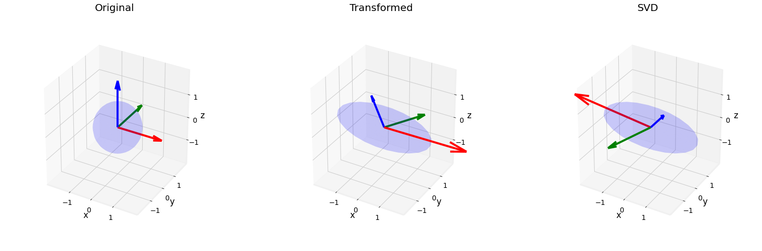
Fig. 2.18 SVD visualization applied to a unit sphere left, with a rotation and stretch matrix transformation middle, and the reconstructed transformation after decomposition by svd (using only $U$ and $\Sigma$).¶

The SVD is particularly useful when the $A$ transformation matrix is rectangular and/or does not allow the computation of its inverse $A^{-1}$. When it is the case, we can compute what is called the Pseudo-Inverse of $A$, $A^+$.

Note

When $A$ is invertible and square, the Economy SVD is the same as the normal SVD.

\[ A^+ A \approx I \; \Rightarrow \; A^+ = V S^{-1} U^T \]

2.8. Applications¶

Linear Algebra is a key concept to represent Applied Mathematics, rigid body physics, fluid mechanics, thermodynamics, computer vision, computer graphics, machine learning, and many others. This section details core example applications of linear algebra and especially the SVD.

2.8.1. Linear System of Equations¶

Let’s considere the Over-Determined System of Linear Equations $A \vec{x} = \vec{b}$ with $A$ an $m \times n$ matrix with $m > n$. Let $\vec{r}$ be the residual for $x$: $\vec{r} = A \vec{x} - \vec{b}$. The vector $\vec{\hat{x}}$ is the one that yields the smallest residual, or more precisely the smallest norm $\|\vec{r}\|$, and is refered as the Least-Squares solution (the best but not unique):

\[ \vec{\hat{x}} = \underset{x \in \mathbb{C}^n}{min} \|\vec{b} - A \vec{x} \| \]

The least-square solution is given by the rewritting the linear system of equation:

\[\begin{split} \begin{equation} \begin{split} A \vec{\hat{x}} & = \vec{b} \\ A^T A \vec{\hat{x}} & = A^T \vec{b} \\ \vec{\hat{x}} & = (A^T A)^{-1} A^T \vec{b} \\ \vec{\hat{x}} & = A^+ \vec{b} \end{split} \end{equation} \end{split}\]

Note

When $\vec{b}$ is null, the system is called an Homogeneous System. In this case, the problem becomes a constraint optimization problem and will not be treated in this chapter.

$A^+$ can be computed easily using its Singular Value Decomposition. Using this method, the system becomes:

\[ \vec{\hat{x}} = A^+ \vec{b} = U \Sigma^+ V^T \vec{b} \]

Let’s try to visualize such as system of equations. Let’s consider 3 planes and let’s find their intersection point:

\[\begin{split} \begin{align} \left\{ \begin{matrix} \begin{split} x & + y & + 0 & = -\frac{1}{2} \\ 0 & + y & + z & = -\frac{1}{2} \\ x & + 0 & + z & = -\frac{1}{2} \\ \end{split} \end{matrix} \right. && \begin{bmatrix} 1 & 1 & 0 \\ 0 & 1 & 1 \\ 1 & 0 & 1 \end{bmatrix} \begin{bmatrix} x \\ y \\ z \end{bmatrix} = \begin{bmatrix} -\frac{1}{2} \\ -\frac{1}{2} \\ -\frac{1}{2} \end{bmatrix} \end{align} \end{split}\]

We can either resolve this system of equations by elimination or using the upper mentionned technique. The solution is:

\[\begin{split} \vec{\hat{x}} = \begin{pmatrix} -\frac{1}{4} \\ -\frac{1}{4} \\ -\frac{1}{4} \end{pmatrix} \end{split}\]

import numpy as np


A = np.array([
    [1.0, 1.0, 0.0],
    [0.0, 1.0, 1.0],
    [1.0, 0.0, 1.0],
])

B = np.array([
    [-0.5],
    [-0.5],
    [-0.5],
])

A_plus = np.linalg.inv(A.T @ A) @ A.T
X = A_plus @ B
print(f"W/ Manual A_plus Computation (inversion):\n{X}\n")

U, S, V_T = np.linalg.svd(A, full_matrices=False)
C = U.T @ B               # U S V_T x = y <=> S V_T x = U_T y = c
W = np.diag(1 / S) @ C    #   S V_T x = c <=> V_T x = 1/S c = w
X = V_T.T @ W             #     V_T x = w <=> x = (V_T)_T w
print(f"W/ Manual Least Square (SVD):\n{X}\n")

X, *_ = np.linalg.lstsq(A, B, rcond=1)
print(f"W/ Numpy Least-square Solver:\n{X}")

W/ Manual A_plus Computation (inversion):
[[-0.25]
 [-0.25]
 [-0.25]]

W/ Manual Least Square (SVD):
[[-0.25]
 [-0.25]
 [-0.25]]

W/ Numpy Least-square Solver:
[[-0.25]
 [-0.25]
 [-0.25]]

from mpl_toolkits.mplot3d import Axes3D
from mpl_toolkits.mplot3d.art3d import Poly3DCollection, Line3DCollection
from shapely.geometry import LineString, Polygon

import numpy as np
import matplotlib.pyplot as plt
plt.ion()
plt.style.use('fivethirtyeight')


def cube_verts(cube: np.ndarray) -> np.ndarray:
    vectors = [*(cube[i] - cube[0] for i in range(1, 3 + 1))]
    verts = cube.tolist()
    verts += [cube[0] + vectors[0] + vectors[1]]
    verts += [cube[0] + vectors[0] + vectors[2]]
    verts += [cube[0] + vectors[1] + vectors[2]]
    verts += [cube[0] + vectors[0] + vectors[1] + vectors[2]]
    return np.array(verts).T
    
    
def cube_edges(verts: np.ndarray) -> np.ndarray:
    return np.array([
        [verts[0], verts[3], verts[5], verts[1]],
        [verts[1], verts[5], verts[7], verts[4]],
        [verts[4], verts[2], verts[6], verts[7]],
        [verts[2], verts[6], verts[3], verts[0]],
        [verts[0], verts[2], verts[4], verts[1]],
        [verts[3], verts[6], verts[7], verts[5]],
    ])


r, c = 2, -0.25

fig = plt.figure(figsize=(8, 8), facecolor="white")
ax = fig.add_subplot(1, 1, 1, projection="3d")

X = cube_verts(np.array((
    (-r, -r, -r),
    (-r,  r, -r),
    ( r, -r, -r),
    (-r, -r,  r),
)))

cube = Poly3DCollection(cube_edges(X.T), linewidths=1, edgecolors='k')
cube.set_facecolor((0, 0, 0, 0.05))
cube.set_edgecolor((0, 0, 0, 1.0))

ax.figure.gca(projection='3d')
ax.add_collection3d(cube)

X, Y = np.meshgrid(range(-r, r + 1), range(-r, r + 1))
Z = np.zeros_like(X) - 0.5
ax.plot_surface(X, Y, Z, color=[1, 0, 0, 0.2])
ax.plot_surface(Z, X, Y, color=[0, 1, 0, 0.2])
ax.plot_surface(X, Z, Y, color=[0, 0, 1, 0.2])

ax.plot([-r, r], [ c, c], [ c, c], linewidth=1, color="r")
ax.plot([ c, c], [-r, r], [ c, c], linewidth=1, color="g")
ax.plot([ c, c], [ c, c], [-r, r], linewidth=1, color="b")

ax.scatter(c, c, c, color="black", marker="+", s=200)

ax.set_xticks(np.arange(-r + 1, r))
ax.set_yticks(np.arange(-r + 1, r))
ax.set_zticks(np.arange(-r + 1, r))
ax.set_xlim(-r, r + 1)
ax.set_ylim(-r, r + 1)
ax.set_zlim(-r, r + 1)
ax.set_xlabel("x")
ax.set_ylabel("y")
ax.set_zlabel("z")
ax.patch.set_facecolor('white')
ax.dist = 12

fig.canvas.draw()

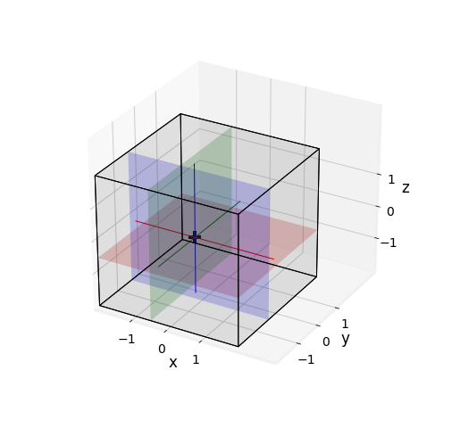
Fig. 2.19 Intersection of 3 planes in $\begin{pmatrix} -\frac{1}{4} \\ -\frac{1}{4} \\ -\frac{1}{4} \end{pmatrix}$.¶

2.8.2. Linear Regression¶

Regression is key to Statistical Analysis tools. It allows us to connect a set of data to another. It consists of finding the line that best model the linear relation between the two sets of data the observation $A$ and the measures $b$, expressed in the model $x$, the unknown.

\[ Ax = b \]

For the sake of sticking with Machine Learning notations, $A$ will be referred to as the target $X$, $b$ ad the output $y$ and $b$ as the weights of the model $w$:

\[ Xw = y \]

A solution to the Linear Regression can be obtained using SVD and solved with the least-squares method:

\[ \hat{w} = X^+ y \]

Note

You can observe that the formulation of the Linear Regression is the same as solving a Linear System of Equation.

Let us observe a one-dimensional example. If we consider a line represented by $3x + 1$, add noise to the line to generate samples, a dataset, and recover the original slope and intercept. In this case, $w$ will contain the slope and intercept numerical, $X$ samples of the perturbed line, and $y$ their corresponding abscissa.

import numpy as np


# Create Targets
original_X = np.linspace(-2, 2, 500)[:, None]
original_y = 3 * original_X + 1

# Create Samples
SAMPLES, NOISE_STRENGTH = 50, (-0.2, 5e-1)
idxs = np.random.choice(len(original_X), SAMPLES)

X, y = original_X[idxs], original_y[idxs]
X += np.random.uniform(*NOISE_STRENGTH, size=len(X))[:, None]    # Add Noise
y += np.random.uniform(*NOISE_STRENGTH, size=len(y))[:, None]    # Add Noise
X = np.column_stack([X, np.ones(len(X))])                        # Add 1 for intercept

# Recover slope and intercept
U, S, V_T = np.linalg.svd(X, full_matrices=False)
w_hat = (V_T.T @ np.diag(1 / S) @ U.T) @ y
print(f"Slope: {w_hat[0, 0]:.2f}\nIntercept: {w_hat[1, 0]:.2f}")

# Prediction
y_preds = X @ w_hat
mse = np.mean((y_preds - y) ** 2)

print(f"MSE: {mse:.2f}")

Slope: 3.02
Intercept: 0.80
MSE: 0.24

import numpy as np
import matplotlib.pyplot as plt
plt.ion()
plt.style.use('fivethirtyeight')

fig = plt.figure(figsize=(4, 4), facecolor="white")
ax = fig.add_subplot(1, 1, 1)

points = ax.scatter(X[:, 0], y[:, 0])
line_origi, *_ = ax.plot(original_X[:, 0], original_y[:, 0])
line_preds, *_ = ax.plot(
    original_X[:, 0],
    w_hat[0, 0] * original_X[:, 0] + w_hat[1, 0],
    color="r",
    linestyle="dashed",
)

ax.set_xlabel("x")
ax.set_ylabel("y")
ax.set_xticks(range(-2, 2 + 1))
ax.legend(
    handles=[points, line_origi, line_preds],
    labels=["noisy data", "true line", "regression line"],
)

fig.canvas.draw()

from myst_nb import glue
glue("matrix_1dlinreg_fig", fig, display=False)

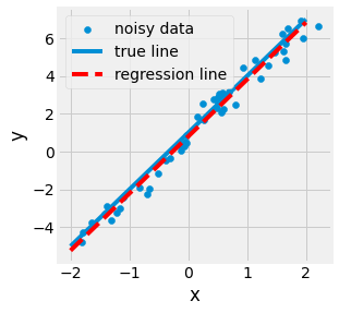
Fig. 2.20 Visualization of a One-dimensional regression for the $3x + 1$ line.¶

Let us observe the classic multi-dimensional dataset Boston. Here, data $X$ represent features of houses such as its area in $m^2$ and $y$ the corresponding median value price in a factor of 1000$. Our goal is to be able to estimate any house price given its available features.

from sklearn.datasets import load_boston
from sklearn.model_selection import train_test_split

import pandas as pd


# Load Boston dataset in memory
data = load_boston(return_X_y=False)

# Split data into train set and test set
X, y = data.data, data.target
X_train, X_test, y_train, y_test = train_test_split(X, y, test_size=0.33, random_state=42)

# Add bias term to the input for learning the line intercept
X_train = np.column_stack([X_train, np.ones(len(X_train))])
X_test = np.column_stack([X_test, np.ones(len(X_test))])

# Show data as a dataframe to display infos table
df = pd.DataFrame(data=X, columns=data.feature_names)
df.head()

	CRIM	ZN	INDUS	NOX	RM	AGE	DIS	RAD	TAX	PTRATIO	B	LSTAT
0	0.00632	18.0	2.31	0.538	6.575	65.2	4.0900	1.0	296.0	15.3	396.90	4.98
1	0.02731	0.0	7.07	0.469	6.421	78.9	4.9671	2.0	242.0	17.8	396.90	9.14
2	0.02729	0.0	7.07	0.469	7.185	61.1	4.9671	2.0	242.0	17.8	392.83	4.03
3	0.03237	0.0	2.18	0.458	6.998	45.8	6.0622	3.0	222.0	18.7	394.63	2.94
4	0.06905	0.0	2.18	0.458	7.147	54.2	6.0622	3.0	222.0	18.7	396.90	5.33

df.info()

<class 'pandas.core.frame.DataFrame'>
RangeIndex: 506 entries, 0 to 505
Data columns (total 13 columns):
 #   Column   Non-Null Count  Dtype  
---  ------   --------------  -----  
 0   CRIM     506 non-null    float64
 1   ZN       506 non-null    float64
 2   INDUS    506 non-null    float64
 3   CHAS     506 non-null    float64
 4   NOX      506 non-null    float64
 5   RM       506 non-null    float64
 6   AGE      506 non-null    float64
 7   DIS      506 non-null    float64
 8   RAD      506 non-null    float64
 9   TAX      506 non-null    float64
 10  PTRATIO  506 non-null    float64
 11  B        506 non-null    float64
 12  LSTAT    506 non-null    float64
dtypes: float64(13)
memory usage: 51.5 KB

import numpy as np


U, S, V_T = np.linalg.svd(X_train, full_matrices=False)
w_hat = (V_T.T @ np.diag(1 / S) @ U.T) @ y_train

y_train_preds = X_train @ w_hat
y_test_preds = X_test @ w_hat

train_mse = np.mean((y_train_preds - y_train) ** 2)
test_mse = np.mean((y_test_preds - y_test) ** 2)

print(f"MSE [train]: {train_mse:.2f}")
print(f"MSE [test ]: {test_mse:.2f}")

MSE [train]: 22.99
MSE [test ]: 20.72

import numpy as np
import matplotlib.pyplot as plt
plt.ion()
plt.style.use('fivethirtyeight')

fig = plt.figure(figsize=(4, 4), facecolor="white")
ax = fig.add_subplot(1, 1, 1)

points = ax.scatter(y_test, y_test_preds)
line, *_ = ax.plot(
    np.linspace(0, 50, 2),
    np.linspace(0, 50, 2),
    color="r",
    linestyle="dashed",
)

ax.set_xlabel("predictions")
ax.set_ylabel("targets")
ax.set_xlim(0, 50)
ax.set_ylim(0, 50)
ax.set_aspect("equal")

fig.canvas.draw()

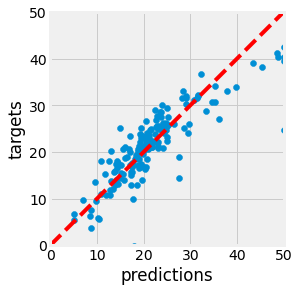
Fig. 2.21 Prediction versus Target in blue. The more the points are close to the dotted line, the better.¶

2.8.3. Image Compression¶

The SVD is also an excellent tool for Image Compression. As the singular values are ordered in $\hat{\Sigma}$ by order of variation represented in the original matrix $A$, by retaining the first $t$ singular values and vectors, $A$ can be compressed. The more singular values are retained, the closer you get to $A$ as you retain higher frequency features. This operation is called a Truncation.

from io import BytesIO
from PIL import Image

import numpy as np
import requests
 

# Load Image in memory from wikipedia and make it grayscale
base = "https://upload.wikimedia.org/wikipedia/commons/d/da/"
url = base + "Athens_coin_discovered_in_Pushkalavati.jpg"
response = requests.get(url)
img = np.array(Image.open(BytesIO(response.content)).convert("L"))

# Compute SVD of the image
U, S, V_T = np.linalg.svd(img, full_matrices=False)

# Compress the Image
truncations = [5, 20, 100]
compressions = [U[:, :t] @ np.diag(S[:t]) @ V_T[:t, :] for t in truncations]

# Compute srotage
to_kB = lambda x: x * 3 / 1024
img_storage = to_kB(np.multiply(*img.shape))

size = lambda U, S, V_T: np.multiply(*U.shape) + len(S) + np.multiply(*V_T.shape)
storages = [to_kB(size(U[:, :t], S[:t], V_T[:t, :])) for t in truncations]

print(f"Original Image: {img_storage:.2f}kB")
for t, s in zip(truncations, storages):
    print(f"SVD Truncation {t}: {s:.2f}kB")

Original Image: 890.62kB
SVD Truncation 5: 17.30kB
SVD Truncation 20: 69.20kB
SVD Truncation 100: 346.00kB

import matplotlib.pyplot as plt
plt.ion()
plt.style.use('fivethirtyeight')

fig = plt.figure(figsize=(8, 4), facecolor="white")
axes = [fig.add_subplot(2, 2, (i % 2) + (i // 2) * 2 + 1) for i in range(4)]

images = [img] + compressions
truncs = [len(V_T)] + truncations
stores = [img_storage] + storages

for i, (ax, img, t, s) in enumerate(zip(axes, images, truncs, stores)):
    ax.imshow(img, cmap="gray")
    ax.set_axis_off()
    if i == 0: ax.title.set_text(f"Original | {s:.2f}kB")
    else: ax.title.set_text(f"T: {t} | {s:.2f}kB")

fig.subplots_adjust(hspace=0.40, wspace=0.25)
fig.canvas.draw()

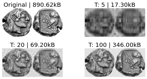
Fig. 2.22 Image Athens coin compressions with SVD and their size in kB. T is the number of singular vectors and values (in order) taken for reconstruction of the image.¶

2.8.4. Principal Component Analysis¶

Principal Component Analysis, or PCA for short, is one of the primary use of the SVD. It consists of constructing a Data-Driven Hierarchical Base within which each orthogonal axis, uncorrelated with each other, represents the main direction, correlation, of the data variation. This process is often referred to as a Dimensionality Reduction technique.

Note

Contrary to what we have used previously throughout this chapter, the data matrix will be considered an array of row vectors instead of column vectors to stay consistent with the statistical PCA literature.

Let the data matrix $X$ of $n \times p$ measurement samples. The first step of the PCA is to considere a Mean-Centered matrix $C$. The mean of a vector is given by:

\[ \tilde{x_{ij}} = \frac{1}{n} \sum_{i=1}^{n} X_{ij} \]

The mean matrix is then:

\[\begin{split} \tilde{X} = \begin{bmatrix} 1 \\ \vdots \\ 1 \end{bmatrix} \tilde{x} \end{split}\]

The mean-centered data matrix is obtained by mean subtraction:

\[ B = X - \tilde{X} \]

The $p \times p$ covariance matrix $C = \frac{1}{n - 1} B^T B$, is symetric and can therefore be diagonalized in the form:

\[ C = V \Lambda V^T \]

The eigenvalues $\lambda_{i}$ present in the diagonal of $\Lambda$ are organized by decreasing order. The corresponding eigenvectors are referred to as the principal directions of the data, and projections of the data on to those principal axes $B \Lambda$ are called principal components, or PC scores.

However, what does it has to do with the SVD? IS this only diagonalization? Well, with a bit of math, one can observe:

\[ C = V \Lambda V^T = V \frac{1}{n - 1} \Sigma^2 V^T \]

and furthermore:

\[ B V = U \Sigma \]

In this sense, the column of $V$ are principal directions, and the column of $U \Sigma$ are the principal components. If we take the first $r$ modes, the first $r$ principal components, we can represent the high $p$-dimensional data matrix as a $r$-dimensional conserving the features’ main correlation.

Let us experiment with this with a toy example to get a first grasp of the PCA.

import numpy as np


means = np.array([2.0, 1.0])    # Gaussian Mean    (x, y)
sigma = np.array([2.0, 0.5])    # Gaussian Stretch (x, y)
theta = 45 * np.pi / 180        # Gaussian Rotation 45 deg
R = np.array([
    [np.cos(theta), -np.sin(theta)],
    [np.sin(theta),  np.cos(theta)],
])

SAMPLES = 10000    # Number of Data points
X = (              # Data Matrix of the Gaussian (2, 1000)
    R @ np.diag(sigma) @ np.random.randn(2, SAMPLES) +
    np.diag(means) @ np.ones((2, SAMPLES))
)

X_mean = X.mean(axis=-1)
B = X - X_mean[:, None]                                                 # Mean Substracted Data Matrix
U, S, V_T = np.linalg.svd(B / np.sqrt(SAMPLES), full_matrices=False)    # PCA via SVD

theta = 2 * np.pi * np.arange(0, 1, 0.01)
X_std = U @ np.diag(S) @ np.array([np.cos(theta), np.sin(theta)])       # Circle representing B std

print(f"Original Sigmas [Data]: {sigma}")
print(f"Infered  Sigmas [SVD] : {S}")

Original Sigmas [Data]: [2.  0.5]
Infered  Sigmas [SVD] : [1.98712996 0.50246625]

import matplotlib.pyplot as plt
plt.ion()
plt.style.use('fivethirtyeight')

fig = plt.figure(figsize=(4, 4), facecolor="white")
ax = fig.add_subplot(1, 1, 1)

ax.scatter(X[0, :], X[1, :])

for i in range(1, 3 + 1):
    ax.plot(X_mean[0] + i * X_std[0, :], X_mean[1] + i * X_std[1, :], color="w", linewidth=2)

for i in range(2):
    x, y = X_mean[0], X_mean[1]
    u, v = X_mean[0] + U[0, i] * S[i], X_mean[1] + U[1, i] * S[i]
    ax.plot([x, u], [y, v], color="r", linewidth=4)
    
ax.set_xlabel("x")
ax.set_ylabel("y")
ax.set_xlim(-6, 8 + 1)
ax.set_ylim(-6, 6 + 1)

fig.canvas.draw()

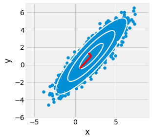
Fig. 2.23 PCA applied to a gaussian toy example in blue. Principal axes are recovered using SVD.¶

Now let us observe the use of PCA on real world data.

from sklearn.datasets import load_breast_cancer
from sklearn.preprocessing import StandardScaler

import pandas as pd
pd.set_option("display.max_columns", 8)


# To Normalize Data (Mean Center and Normalize Variation)
sc = StandardScaler()

# Load Breast Cancer dataset in memory
data = load_breast_cancer(return_X_y=False)
X, y = sc.fit_transform(data.data), data.target

# Show data as a dataframe to display infos table
df = pd.DataFrame(data=X, columns=data.feature_names)
df.head()

	mean radius	mean texture	mean perimeter	mean area	...	worst concavity	worst concave points	worst symmetry	worst fractal dimension
0	1.097064	-2.073335	1.269934	0.984375	...	2.109526	2.296076	2.750622	1.937015
1	1.829821	-0.353632	1.685955	1.908708	...	-0.146749	1.087084	-0.243890	0.281190
2	1.579888	0.456187	1.566503	1.558884	...	0.854974	1.955000	1.152255	0.201391
3	-0.768909	0.253732	-0.592687	-0.764464	...	1.989588	2.175786	6.046041	4.935010
4	1.750297	-1.151816	1.776573	1.826229	...	0.613179	0.729259	-0.868353	-0.397100

5 rows × 30 columns

df.info()

<class 'pandas.core.frame.DataFrame'>
RangeIndex: 569 entries, 0 to 568
Data columns (total 30 columns):
 #   Column                   Non-Null Count  Dtype  
---  ------                   --------------  -----  
 mean radius              569 non-null    float64
 mean texture             569 non-null    float64
 mean perimeter           569 non-null    float64
 mean area                569 non-null    float64
 mean smoothness          569 non-null    float64
 mean compactness         569 non-null    float64
 mean concavity           569 non-null    float64
 mean concave points      569 non-null    float64
 mean symmetry            569 non-null    float64
 mean fractal dimension   569 non-null    float64
radius error             569 non-null    float64
texture error            569 non-null    float64
perimeter error          569 non-null    float64
area error               569 non-null    float64
smoothness error         569 non-null    float64
compactness error        569 non-null    float64
concavity error          569 non-null    float64
concave points error     569 non-null    float64
symmetry error           569 non-null    float64
fractal dimension error  569 non-null    float64
worst radius             569 non-null    float64
worst texture            569 non-null    float64
worst perimeter          569 non-null    float64
worst area               569 non-null    float64
worst smoothness         569 non-null    float64
worst compactness        569 non-null    float64
worst concavity          569 non-null    float64
worst concave points     569 non-null    float64
worst symmetry           569 non-null    float64
worst fractal dimension  569 non-null    float64
dtypes: float64(30)
memory usage: 133.5 KB

from sklearn.decomposition import PCA


# Sklearn PCA
sk_pca = PCA(n_components=2).fit(X)    # Compute PCA via SVD or Eigen Vectors
sk_pca_X = sk_pca.fit_transform(X)     # Project Data on first 2 modes

# Manual PCA
p, n = X.shape
U, S, V_T = np.linalg.svd(X, full_matrices=False)    # Compute PCA via SVD
m_pca_X = (X @ V_T.T[:, :2])                         # Project Data on first 2 modes

import matplotlib.pyplot as plt
plt.ion()
plt.style.use('fivethirtyeight')

fig = plt.figure(figsize=(8, 4), facecolor="white")
ax1, ax2 = [fig.add_subplot(1, 2, i + 1) for i in range(2)]

ax1.semilogy(S)
ax1.set_xlabel("r")
ax1.set_ylabel("singular value r")

ax2.plot(np.cumsum(S) / np.sum(S))
ax2.set_xlabel("r")
ax2.set_ylabel("cumulative energy")

fig.subplots_adjust(hspace=0.25, wspace=0.40)
fig.canvas.draw()

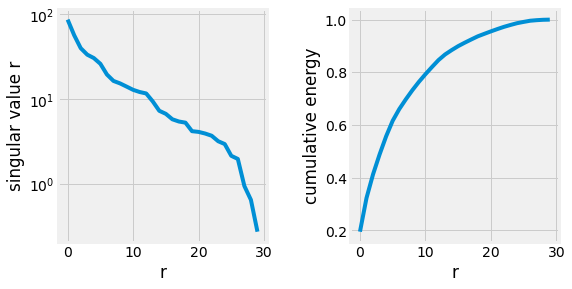
Fig. 2.24 Singular values of the Breast Cancer Dataset.¶

import matplotlib.pyplot as plt
plt.ion()
plt.style.use('fivethirtyeight')


def plot_data(ax: plt.Figure, pca_X: np.ndarray, y: np.ndarray) -> None:
    lc, ln = False, False    # Ensure only one label for legend
    for coords, label in zip(pca_X, y):
        c = "r" if label else "#008FD5"
        m = "<" if label else "o"

        l = "Cancer" if label else "Normal"
        if l == "Cancer" and not lc: lc = True
        elif l == "Normal" and not ln: ln = True
        else: l = "_"
            
        ax.scatter(*coords, color=c, marker=m, alpha=0.5, label=l)
    ax.set_xlabel("PCA 1")
    ax.set_ylabel("PCA 2")
    ax.legend()



fig = plt.figure(figsize=(8, 4), facecolor="white")
ax1, ax2 = [fig.add_subplot(1, 2, i + 1) for i in range(2)]

plot_data(ax1, sk_pca_X, y)
ax1.title.set_text("sklearn PCA")

plot_data(ax2, m_pca_X, y)
ax2.title.set_text("manual PCA")

fig.subplots_adjust(hspace=0.25, wspace=0.40)
fig.canvas.draw()

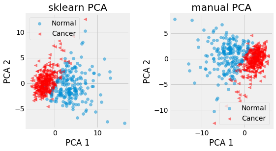
Fig. 2.25 First 2 principal components of the Breast Cancer dataset provided by sklearn. Cancer patients are represented in red, and normal ones in blue. Notice the sign difference between the manual PCA (using svd) and the sklearn one. This is due to the fact that eigenvectors represent the direction of a span which is invariant to its sign.¶

2.8.5. Eigenfaces¶

A great example of the use of SVD and PCA is the Eigenfaces. An eigenface is a set of eigenvectors used for Face Recognition. The approach was first developed by Sirovich and Kirby in 1987 and used by Matthew Turk and Alex Pentland for face classification. As shown with PCA, the eigenvectors are derived from the covariance matrix describing all the face images’ high-dimensional space. Any face can then be reconstructed using this basis, and not only faces.

Note

The problem of Eigenfaces is left to the student. Solutions are given by unhiding the corresponding code. As always, try to do it yourself before giving a glance at the answers. Try to make your brain actively recovering this entire chapter.

The dataset used for the example is Labeled Faces in the Wild, or LFW for short. The version of the dataset sklearn provides is a subset of the full dataset, which contains 1288 samples of 62x47 face images from 7 people.

The code to load the dataset is provided below:

from sklearn.datasets import fetch_lfw_people

import numpy as np


# Fetch LFW Dataset
lfw_people = fetch_lfw_people(min_faces_per_person=70)
n_samples, h, w = lfw_people.images.shape

# Get data matrix X (h * w, n) and y (n, )
X, y = lfw_people.data.T, lfw_people.target
n_features, n_classes = X.shape[0], len(np.unique(y))
print(f"Samples: {n_samples}, Features: {n_features}, Classes: {n_classes}")

# Split in train and test set
train_candidates = y < 5
test_candidates = y >= 5

X_train, y_train = X[:, train_candidates], y[train_candidates]
X_test, y_test = X[:, test_candidates], y[test_candidates]

Samples: 1288, Features: 2914, Classes: 7

2.8.5.1. Decomposition¶

First, start by computing and visualizing the eigenfaces, their energy, and how they look by applying the decomposition techniques studied in this chapter.

import numpy as np


# Compute Mean Face to Mean Center the data matrix
X_mean = X_train.mean(axis=-1)
B_train = X_train - X_mean[:, None]

# Apply SVD to capture Principal Components (U is array of column eigen vectors/faces)
U, S, V_T = np.linalg.svd(B_train, full_matrices=False)

import matplotlib.pyplot as plt
plt.ion()
plt.style.use('fivethirtyeight')

fig = plt.figure(figsize=(8, 4), facecolor="white")
ax1, ax2 = [fig.add_subplot(1, 2, i + 1) for i in range(2)]

ax1.semilogy(S)
ax1.set_xlabel("r")
ax1.set_ylabel("eigen value r")

ax2.plot(np.cumsum(S) / np.sum(S))
ax2.set_xlabel("r")
ax2.set_ylabel("cumulative enery")

fig.subplots_adjust(hspace=0.25, wspace=0.40)
fig.canvas.draw()

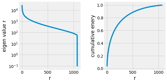
Fig. 2.26 Singular values of the Eigenfaces.¶

import matplotlib.pyplot as plt
plt.ion()
plt.style.use('fivethirtyeight')

fig = plt.figure(figsize=(12, 4), facecolor="white")
ax1 = fig.add_subplot(1, 2, 1)

ax1.imshow(X_mean.reshape(h, w), cmap="gray")
ax1.set_axis_off()
ax1.title.set_text("Mean Face")

for i in range(3):
    for j in range(3):
        idx = i + j * 3
        ax = fig.add_subplot(3, 6, 3 * (j + 1) + i + j * 3 + 1)
        ax.imshow(U[:, idx].reshape(h, w), cmap="gray")
        ax.set_axis_off()
        ax.title.set_text(f"Eigenface {idx + 1}")

fig.subplots_adjust(hspace=0.40, wspace=0.40)
fig.canvas.draw()

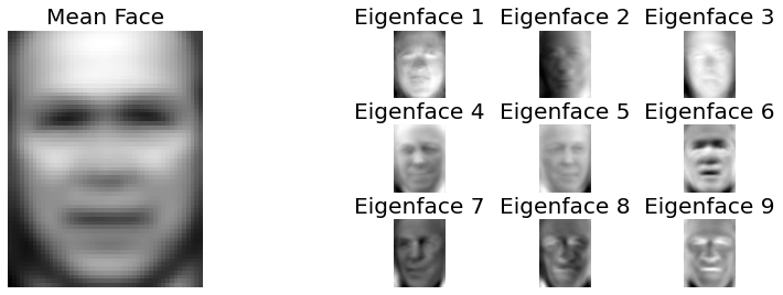
Fig. 2.27 Mean face of the LFW dataset and the first 9 eigen faces.¶

2.8.5.2. Approximation¶

Then try to approximate the two remaining faces using the computed eigenfaces, and visualize their appearance depending on different truncations.

Note

Remember $U^T=U^{-1}$ as $U$ is defined as an otheogonal matrix. A consequence of this fact is $X=U U^T X$.

# Facial Reconstructions for test Candidate 0
X_candidate = X_test[:, 0]
B_candidate = X_candidate - X_mean

modes = [25, 50, 100, 150, 300]
recons = [X_mean + U[:, :r] @ U[:, :r].T @ B_candidate for r in modes]

import matplotlib.pyplot as plt
plt.ion()
plt.style.use('fivethirtyeight')

fig = plt.figure(figsize=(12, 8), facecolor="white")

for i, (r, recon) in enumerate(zip([n_features] + modes, [X_candidate] + recons)):
    ax = fig.add_subplot(3, 3, (i % 3) + (i // 3) * 3 + 1)
    ax.imshow(recon.reshape(h, w), cmap="gray")
    ax.set_axis_off()
    ax.title.set_text("Original" if i == 0 else f"r: {r}")

fig.subplots_adjust(hspace=0.40, wspace=0.25)
fig.canvas.draw()

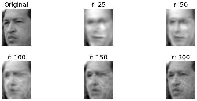
Fig. 2.28 Approximate representations of the first test candidate using the eigenfaces.¶

Try to approximate an image completely different from the one present in the dataset, a coin, for example.

from io import BytesIO
from PIL import Image

import requests
 

# Load Image in memory from wikipedia and make it grayscale
url = "https://upload.wikimedia.org/wikipedia/commons/3/3b/Claudius_II_coin_%28colourised%29.png"
response = requests.get(url)
coin = np.array(Image.open(BytesIO(response.content)).convert("L").resize((w, h)))

# Reshape data to feature vector
X_coin = coin.reshape(-1)

# Candle Reconstructions
B_coin = X_coin - X_mean

modes = [25, 50, 100, 150, 300]
recons = [X_mean + U[:, :r] @ U[:, :r].T @ B_coin for r in modes]

import matplotlib.pyplot as plt
plt.ion()
plt.style.use('fivethirtyeight')

fig = plt.figure(figsize=(12, 8), facecolor="white")

for i, (r, recon) in enumerate(zip([n_features] + modes, [X_coin] + recons)):
    ax = fig.add_subplot(3, 3, (i % 3) + (i // 3) * 3 + 1)
    ax.imshow(recon.reshape(h, w), cmap="gray")
    ax.set_axis_off()
    ax.title.set_text("Original" if i == 0 else f"r: {r}")

fig.subplots_adjust(hspace=0.40, wspace=0.25)
fig.canvas.draw()

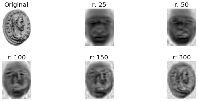
Fig. 2.29 Approximate representations of the Claudius II Coin using the eigenfaces.¶

2.8.5.3. Embedding¶

Finally, try to represent the two remaining faces on two contiguous eigenfaces basis axes and visualize it.

# Get Faces from test Candidates and Project on PCA 3 and 4
B_test = X_test - X_mean[:, None]
pca_B = U[:, 2:4].T @ B_test

import matplotlib.pyplot as plt
plt.ion()
plt.style.use('fivethirtyeight')

fig = plt.figure(figsize=(12, 4), facecolor="white")
ax1, ax2, ax3 = [fig.add_subplot(1, 3, i + 1) for i in range(3)]

for ax, idx in zip([ax1, ax3], [5, 6]):
    ax.imshow(X_test[:, (y_test == idx)][:, 0].reshape(h, w), cmap="gray")
    ax.set_axis_off()
    ax.title.set_text(f"Candidate {idx - 5 + 1}")

ax2.scatter(*pca_B[:, (y_test == 5)], marker="o")
ax2.scatter(*pca_B[:, (y_test == 6)], marker="v")
ax2.legend(labels=[f"Candidate {i}" for i in [1, 2]])
ax2.set_xlabel("pca 3")
ax2.set_ylabel("pca 4")
ax2.set_xticks([0,])
ax2.set_yticks([0,])

fig.subplots_adjust(hspace=0.25, wspace=0.40)
fig.canvas.draw()

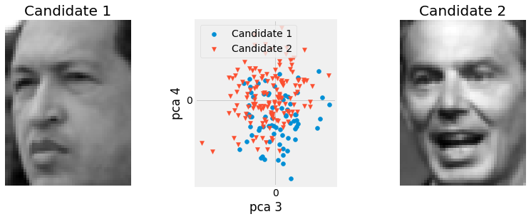
Fig. 2.30 Projection of the 2 test candidates on to the 4th and 3rd principal components. Their projection almost allow us to cluster them visually, although it is not perfect due parlty to the lack of feature alignement in the chosen dataset.¶

Data-Driven Science: a Python Visual and Practical Text Book

2. Linear Algebra¶

2.1. Introduction¶

2.2. Fundamental Objects¶

2.2.1. Scalars¶

2.2.2. Vectors¶

2.2.2.1. Magnitude and Unit Vector¶

2.2.2.2. Scaling and Addition¶

2.2.2.3. Dot Product¶

2.2.2.4. Cross Product¶

2.2.3. Matrices¶

2.2.3.1. Scaling and Addition¶

2.2.3.2. Transpose¶

2.2.3.3. Hadamard Product¶

2.2.3.4. Matrix Multiplication¶

2.3. Square Matrices¶

2.3.1. Diagonal and Triangular Matrices¶

2.3.2. Identity¶

2.3.3. Special Square Matrices¶

2.3.4. Trace¶

2.3.5. Determinant¶

2.4. Linear Transformations¶

2.4.1. Scale¶

2.4.2. Rotation¶

2.4.3. Shearing¶

2.4.4. Reflection¶

2.5. Affine Transformations¶

2.5.1. Tranlsation¶

2.6. Eigenvectors and Diagonalization¶

2.6.1. Eigenvector¶

2.6.2. Diagonalisation¶

2.7. Singular Value Decomposition¶

2.8. Applications¶

2.8.1. Linear System of Equations¶

2.8.2. Linear Regression¶

2.8.3. Image Compression¶

2.8.4. Principal Component Analysis¶

2.8.5. Eigenfaces¶

2.8.5.1. Decomposition¶

2.8.5.2. Approximation¶

2.8.5.3. Embedding¶