
4. Statistical Inference
4.1. Introduction
Statistical Inference uses classical statistics to observe, study, and predict patterns resulting from data analysis and probabilistic modeling. There are two main approaches to the field, either Frequentist or Bayesian. The first approach implies a fixed distribution responsible for the generation of repeated patterns in the data. We can find the best estimate of the distribution’s parameters given data samples. The last one implies that the state of the world can be updated using observed samples. The parameters of the distributions can themselves be represented using probability.
As an example, here is a situation explaining using the two frameworks. Imagine your phone is ringing in your house, and you want to reach it:
Frequentist: I have a mental model of my house. Given the beeping sound, I can infer the house’s area to search for my phone.
Bayesian: On top of having a mental model of my house, I also remember from the past where I misplaced the phone. By combining my inferences using the beeps and my prior information on its location, I can identify the house area and locate my phone.
4.2. Statistical Analysis Fundamentals
Statistical Analysis allows us to describe patterns observed in any given dataset via Visualization or Statistical Descriptors. In statistics, we are interested in studying a given Sample from a Population of Individuals.
Note
Statistical Descriptors are closely related to Probability Descriptors. As we will observe later in the chapter, the Observed Mean can be associated with the Expectation, the Observed Variance to the Variance, and many more.
Suppose we design a study on the effectiveness of some medicine for some given disease. In that case, the sample corresponds to the set of patients who participated in the study, and the population represents all the people suffering from the studied disease.
To give credit to a Study, in other word to Generalize its results, the sample needs to Reflect the Variation present in the entire population of interest. One way to obtain such a sample is to include Randomness in the population’s selection process.
Now that we have defined the context of application let us define all the fundamentals of Statistical Analysis.
Note
The different types of visualizations that can be used to express some data series’ underlying variations have been discussed in the Data Visualization Chapter.
4.2.1. Central Tendency
The first type of descriptor is the Central Tendency. It expresses the central value, the typical value for a data distribution. The most common central tendency measures are the Mode, the Mean, and the Median.
The Mode \(M_o\) is the value that occurs most often in a given set of data values.
The Mean \(\overline{x}\) refers to the Arithmetic Mean:
In some cases it also refers to the Weighted Arithmetic Mean:
The Median \(M_e\) is the variable responsible for separating the statistical distributions as two equally populated groups when organized in ascending order.
Let us consider the following example, which compiles one exam score for each of \(22\) students and compute its central tendency metrics:
import pandas as pd
import numpy as np
np.random.seed(42)
pd.options.display.max_columns = 22


N = 22

# Generate Data for Example
df = pd.DataFrame(data=np.random.normal(13, 3, size=N).astype(int), columns=["score"])
df.head(N).T
| 0 | 1 | 2 | 3 | 4 | 5 | 6 | 7 | 8 | 9 | 10 | 11 | 12 | 13 | 14 | 15 | 16 | 17 | 18 | 19 | 20 | 21 | |
|---|---|---|---|---|---|---|---|---|---|---|---|---|---|---|---|---|---|---|---|---|---|---|
| score | 14 | 12 | 14 | 17 | 12 | 12 | 17 | 15 | 11 | 14 | 11 | 11 | 13 | 7 | 7 | 11 | 9 | 13 | 10 | 8 | 17 | 12 |
print(f"Mode  : {df.score.mode().array[0]:.2f}")
print(f"Mean  : {df.score.mean():.2f}")
print(f"Median: {df.score.median():.2f}")
Mode  : 11.00
Mean  : 12.14
Median: 12.00
import matplotlib.pyplot as plt
import numpy as np
plt.ion()
plt.style.use('fivethirtyeight')

fig = plt.figure(figsize=(8, 4), facecolor="white")
ax = fig.add_subplot(1, 1, 1)

ax.hist(df.score, bins=np.arange(20) - 0.5, rwidth=0.9)
line1 = ax.axvline(df.score.mode().array[0], color="#E5AE42", linestyle="--")
line2 = ax.axvline(df.score.mean(), color="#F6514C", linestyle="--")
line3 = ax.axvline(df.score.median(), color="k", linestyle="--")
ax.set_xlabel("score")
ax.set_ylabel("count")
ax.set_xticks(range(0, 20 + 1, 2))
ax.set_xlim(-0.5, 20.5)
ax.legend(handles=[line1, line2, line3], labels=["Mode", "Mean", "Median"])

fig.canvas.draw()
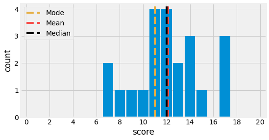
Fig. 4.1 Mode, Mean, and Median Visualization for a dataset containing exam’s scores of \(22\) students.
4.2.2. Spread
The second type of descriptor is the Spread or Dispersion of a data series. It is often implied to be the spread around its mean. The most common spread measures are the Range and the Variance, thus the Standard Deviation.
The Range \(R\) of a data series is defined as the difference between its maximum and minimum values. If the values are organized in ascending order, its:
The Variance, \(s^2\) for some observed data series, \(\sigma^2\) for some theoretical distribution, is the average sum of square difference from the mean. It explains how the data is distributed around the mean. The Standard Deviation is defined as the square root of the variance. It allows working with the same unit as the data.
Let us consider the same example as for the central tendency and compute the range and the standard deviation of the student scores:
print(f"Range: {df.score.max() - df.score.min():.2f}")
print(f"Std  : {df.score.std():.2f}")
Range: 10.00
Std  : 2.93
4.2.3. Correlation
The last type of descriptor is the Correlation between two variables \(X\) and \(Y\). In satistical analysis, it is often easier to interpret the correlation between two variables of the same unit. If it is not the case, it is common practice to centre and reduce the variables \(x = \frac{X - \mu}{\sigma}\).
One of the correlation metrics is the Linear Correlation Coeficient between \(X\) and \(Y\) and is defined as:
When \(\rho(X, Y)\) is closed to \(-1\) or \(1\), it means that \(X\) and \(Y\) are linearly related, and the sign defines the direction of the linearity. If \(\rho(X, Y)\) is null, there is no linear dependency, no correlation between the two variables.
import matplotlib.pyplot as plt
import numpy as np
plt.ion()
plt.style.use('fivethirtyeight')
np.random.seed(42)

N = 100

fig = plt.figure(figsize=(12, 4), facecolor="white")
ax1, ax2, ax3 = [fig.add_subplot(1, 3, i + 1) for i in range(3)]

XY = np.random.normal(0, 1, (N, 2))
ax1.scatter(XY[:, 0], XY[:, 1])
ax1.set_axis_off()
ax1.title.set_text(r"$\rho$=0")

ax2.scatter(XY[:, 0], XY[:, 0])
ax2.set_axis_off()
ax2.title.set_text(r"$\rho$=1")

ax3.scatter(XY[:, 0], -XY[:, 0])
ax3.set_axis_off()
ax3.title.set_text(r"$\rho$=-1")

fig.subplots_adjust(hspace=0.40, wspace=0.25)
fig.canvas.draw()
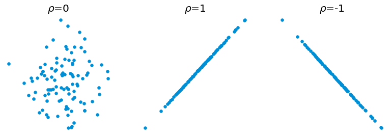
Fig. 4.2 Visualization of the linear correlation coeficient between \(X\) and \(Y\).
4.3. Sampling and Central Limit Theorem
4.3.1. Sample
As stated previously in the chapter, statistic analysis allows us to study some probabilistic phenomena, for example, the error in diameter of a milling machine, on a defined Sample as the statistical characteristics of an entire population cannot be measured. In statistics, a Sample has to represent a maximum of the variance present in the population it is drawn from using a known distribution.
A Sample can be defined as a set of \(n\) independant random variable \((X_1,\cdots,X_n)\) drawn from a same distribution. The Observations of a the sample are defined by \((x_1,\cdots,x_n)\).
A Statistic \(T\) is a quantity, a measurable function, from the sample’s values.
The Empirical Mean Satistic \(\overline{X}_n\) is:
If we define \(\mu\) the expected value, and \(\sigma^2\) the variance of the random variable \(X\), the Expected Value and the Variance for the statistic \(\overline{X}_n\) can be defined as:
4.3.2. Central Limit Theorem
In this section, two fundamental theorems of statistics are discussed, the Law of Large Numbers and the Central Limit Theorem. Both of them concern the \(\overline{X}_n\) statistic for samples of independent and identically distributed random variables.
The Law of Large Numbers states that for such a framework, as the sample size grows, its mean gets closer to the average of the entire population. We have been relying secretly on this theorem when dealing with Monte Carlo Simulation.
Let us verify this fact empirically with an example. Consider a dice where \(X\) represents the outcome number of a throw and follows a uniform distribution.
Let us repeat the experiment \(n\) times and compute the statistic \(\overline{X}_n\). When the sample size grows, its value should be closer to \(\mu\), which is \(3.5\). It is visually possible to verify that this convergence happens.
import matplotlib.pyplot as plt
import numpy as np
plt.ion()
plt.style.use('fivethirtyeight')
np.random.seed(42)

fig = plt.figure(figsize=(8, 4), facecolor="white")
ax = fig.add_subplot(1, 1, 1)

line1, *_ = ax.plot([np.random.uniform(1, 6, n).mean() if n > 0 else 0 for n in range(500)])
line2, *_ = ax.plot(np.ones(500) * 3.5, color="#F6514C", linestyle="--")
ax.legend(handles=[line1, line2], labels=["$\overline{X_n}$", "$\mu$ = 3.5"])
ax.set_xlabel("n")
ax.set_ylabel("X")
ax.set_ylim(-0.2, 6.2)

fig.canvas.draw()
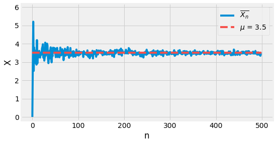
Fig. 4.3 Visualization of the Low of Large Numbers. When \(n\) grow, \(\overline{X}_n\) gets closer to \(\mu\).
The Central Limit Theorem States that for such a framework as the one described for this section, with expectation \(\mu\) and variance \(\sigma^2\):
To resume, for any sample of a reasonably big size of independent random variable \(X_i\), the standardized mean distribution \(Z\) can be simplified to a normal distribution \(\mathcal{N}(0, 1)\).
Let us verify this fact empirically with an example. Consider the uniform distribution \(U(0, 1)\) and the poisson distribution \(Pois(1)\). By taking samples of bigger and bigger sizes, the distribution of \(\overline{X}_n\) should resemble the one of a normal distribution.
import matplotlib.pyplot as plt
import numpy as np
import seaborn as sns
plt.ion()
plt.style.use('fivethirtyeight')
np.random.seed(42)

sizes = [1, 5, 10, 50]
samples = 400

fig = plt.figure(figsize=(len(sizes) * 4, 8), facecolor="white")

for i, n in enumerate(sizes):
    ax = fig.add_subplot(2, len(sizes), i + 1)
    X_n = np.random.uniform(0, 1, (samples, n)).mean(-1)
    sns.histplot(X_n, kde=True, ax=ax)
    ax.set_ylim(-0.5, 70.5)
    ax.set_xlim(0, 1)
    ax.set_xticks((0, 0.5, 1))
    ax.set_yticks(())
    ax.grid()
    if i > 0: ax.set_ylabel("")
    else: ax.set_ylabel("U(0, 1)")
    ax.title.set_text(f"n = {n}")

for i, n in enumerate(sizes):
    ax = fig.add_subplot(2, len(sizes), len(sizes) + i + 1)
    X_n = np.random.poisson(1.0, (samples, n)).mean(-1)
    sns.histplot(X_n, kde=True, ax=ax)
    ax.set_ylim(-0.5, 200.5)
    ax.set_xlim(0, 2)
    ax.set_xticks((0, 1, 2))
    ax.set_yticks(())
    ax.grid()
    if i > 0: ax.set_ylabel("")
    else: ax.set_ylabel("Pois(1)")

fig.canvas.draw()
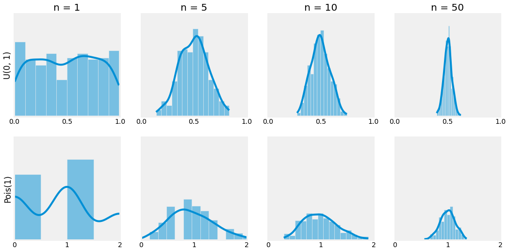
Fig. 4.4 Visualization of the Central Limit Theorem. When \(n\) grow, the distribution of \(\overline{X}_n\) gets closer to a normal distribution.
4.4. Estimates
The goal of statistical inference is to find, to infer, some Estimate of some Parameters \(\theta\) governing some hypothetical distribution supposed to be responsible for the variation in the set of random variables studied \(X\). The distribution is chosen appropriately using the tools of statistical analysis.
The idea of an Estimator is to approximate a statistical parameter. Statistical descriptors are such estimators as they approximate a statistical parameter concerning the studied population given a sample. An Estimate is the value obtained after the measurement of an estimator.
As it may imply in its name, approximate means that an estimate is not and never will be perfect. There is some notion of error, commonly referred to as the Margin of Error.
In this section, we study two different kinds of estimators, Point Estimators and Interval Estimators, and discuss approaches to find them.
4.4.1. Point Estimate
Point Estimators can be created using different approaches. Among them three will be presented, the Method of Moments, the Maximum Likelihood Estimation, and the Maximum a Posteriori Estimation.
Note
Unkown Population Parameter |
Symbol |
Empirical Point Estimation |
Symbol |
|---|---|---|---|
Population mean |
\(\mu\) |
Sample mean |
\(\hat{\mu}\) |
Population standard deviation |
\(\sigma^2\) |
Sample variance |
\(\hat{\sigma}^2\) |
Population standard deviation |
\(\sigma\) |
Sample standard deviation |
\(\hat{\sigma}\) |
Population proportion |
\(p\) |
Sample proportion |
\(\hat{p}\) |
4.4.1.1. Method of Moments (MM)
Before even looking at the Method of Moments, or MM for short, we need to define a Moment. The \(k\)-th Moment of a given random variable \(X\) is expressed as:
We already know from now on that an approximation of the first moment of \(X\) is given by the sample mean:
Base on that we can approximate hte \(k\)-th Moment of \(X\) by:
Let us consider the following example. Considere the random sample \(X_1, \dots, X_n\) and try to approximate the population mean \(\mu = \mathbb{E}[X]\) and the variance of the popylation \(\sigma^2 = \mathbb{E}[(X - \mathbb{E}[X])^2] = \mathbb{E}[X^2] - \mu^2\) using the method of moments:
As you can notice, the method revolves around the sample mean and does not require any PDF nor PMF computation. One downfall of this method can be observed by looking at the second term of the variance estimator. If this term is too big, the approximation result will be negative, which is not acceptable.
4.4.1.2. Maximum Likelihood Estimation (MLE)
Another method for creating point estimators is the Maximum Likelihood. Let us remind the context we are dealing with. Consider \(X_1, \dots, X_n\) a random sample (independent) of size \(n\) sampled from a PDF or PMF \(p(D | \theta)\). Our goal is to estimate, approximate \(\theta\). In this sense, we want to find:
This method, as its name implies, consists on maximizing a function \(\mathcal{L}(\theta | X_1, \dots, X_n)\) representing the Likelihood of having \(\theta\) given our sample. The Likelihood Function is defined as the joint PMF of each individual of our sample:
The parameter \(\hat{\theta}\) that maximizes the likelihood function is called the Maximum Likelihood Estimator, or MLE for short. As a reminder, finding the maximum of some function \(f\) can be done by studying its derivative \(f'\). In this sense we will often talk about the Log Likelihood Function:
Log is a Monotonic function, it does not change the order of what it is given, and the log of a product is the sum of logs. It allows us to simplify the likelihood as a sum and thus to simplify the process of derivation.
Consider the following example: you are playing basket ball and after 15 independent throws, only 6 made it. Let denot \(X\) the number of successes. With this formulation, \(x=6\) and \(n=15\). Now let us assume that \(X \sim B(n, \theta)\) and estimate \(\theta\) by computing its MLE.
After solving the equation \(l'(X | \theta) = 0\), we obtain the following root: \(\hat{\theta} = \frac{X}{n}\). If we evaluate this estimator, we obtain the Maximum Likelihood Estimate \(\hat{\theta} = \frac{6}{15}\).
from torch.autograd import Variable
from typing import List

import numpy as np
import torch
torch.manual_seed(42)
np.random.seed(42)


# Replicate Trial (15 Throws, 6 Successes)
n = 15
shuffle = lambda _: np.random.rand()
observations = sorted([1] * 6 + [0] * (n - 6), key=shuffle)
observations = torch.Tensor(observations).float()


# Define Bernoulli Model
class BernoulliModel:
    def __init__(self) -> None:
        """Bernoulli Model
        p = theta  is unknown and initialized to 0.5
        """
        self.p = Variable(torch.tensor(0.5), requires_grad=True)

    def __call__(self, x: torch.Tensor) -> torch.Tensor:
        """Bernoulli PMF
        p^x (1 - p)^(1 - x)
        """
        return (self.p ** x) * ((1.0 - self.p) ** (1.0 - x))

    def fit(
        self, observations: torch.Tensor,
        iterations: int = 10, lr: float = 1e-1,
    ) -> List[float]:
        """Maximum Likelihood Estimation
        Optimization -> Gradient Ascent (find max using derivative)
        """
        history = [self.p.item()]
        for iteration in range(iterations):
            loglikelihood = torch.mean(torch.log(self(observations)))
            loglikelihood.backward()

            self.p.data.add_(lr * self.p.grad.data)
            self.p.grad.data.zero_()
            print(f"Iteration {iteration}: 𝑝̂={self.p.item():.2f}")

            history.append(self.p.item())
        return history


# Statistical Inference using MLE
model = BernoulliModel()
history = model.fit(observations)
Iteration 0: 𝑝̂=0.46
Iteration 1: 𝑝̂=0.44
Iteration 2: 𝑝̂=0.42
Iteration 3: 𝑝̂=0.41
Iteration 4: 𝑝̂=0.41
Iteration 5: 𝑝̂=0.40
Iteration 6: 𝑝̂=0.40
Iteration 7: 𝑝̂=0.40
Iteration 8: 𝑝̂=0.40
Iteration 9: 𝑝̂=0.40
import matplotlib.pyplot as plt
import seaborn as sns
plt.ion()
plt.style.use("fivethirtyeight")

fig = plt.figure(figsize=(8, 4),  facecolor="white")
ax1, ax2 = [fig.add_subplot(1, 2, i + 1) for i in range(2)]

sns.histplot(observations, ax=ax1, stat="probability", discrete=True)
ax1.set_ylim(0, 1)
ax1.set_xticks([0, 1])
ax1.title.set_text("Sample")
ax1.set_xlabel("x")
ax1.set_ylabel("proportion")
ax1.grid(axis='x')

ax2.plot(history)
ax2.title.set_text("MLE")
ax2.set_xlabel("step")
ax2.set_ylabel("$\hat{p}$")

fig.subplots_adjust(hspace=0.25, wspace=0.40)
fig.canvas.draw()
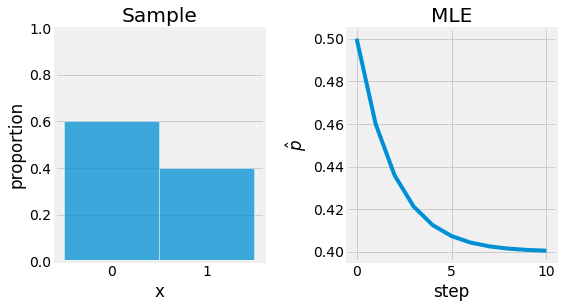
Fig. 4.5 Maximum Likelihood Estimate applied to the basket ball throw example. The objective is to find \(p\) for \(B(n, p)\). Sample is represented left, and the optimization process base on the MLE right.
4.4.1.3. Maximum a Posteriori Estimation (MAP)
The last method presented in this section is the Maximum a Posteriori Estimation (MAP). It is similar and related to the Maximum Likelihood Estimate but considers a posterior knowledge on the parameters we want to estimate. The method can be derived from the MLE using Baye’s Theorem.
This technique assume the same setup of \(n\) random independent samples \(X_1, \dots, X_n\). Our goal is to find a good estimate of some parameters \(\theta\) for the given dataset. Contrary to MLE, MAP consider the best estimate as beign drawn from \(p(\theta|D)\):
Instead of maximizing the likelihood function, here, we maximize a posterior distribution on the parameters.
The same process used for MLE can now be applied. It is just a matter of finding the maximum of this function by computing its derivative. It means that our best estimate \(\theta_{MAP}\) is the most probable \(\theta\) given observed data and our prior belief. It can be seen as a compromise between the likelihood and posterior belief.
Let us now reconsidere the example of basketball throws. This time let us consider some prior knowlege on the parameter \(\theta\), the estimator of \(p\) in \(B(n, p)\). Assuming \(\theta\) follows a Beta distribution \(P(\theta) \sim Beta(\alpha, \beta)\):
Using this knowledge:
If we look closely, we can observe that \(P(\theta|X) \sim Beta(X + \alpha, n - X + \beta)\). Thus:
Solving \(l'(\theta | X)=0\) gives us \(\hat{\theta} = \frac{X + \alpha - 1}{\alpha + n + \beta - 2}\). If we choose a prior with \(\alpha=0.7\), and \(\beta=0.8\), \(\hat{\theta} \approx 0.41\).
from scipy.special import gamma
from torch.autograd import Variable
from typing import Callable, List

import numpy as np
import torch
torch.manual_seed(42)
np.random.seed(42)


# Replicate Trial (15 Throws, 6 Successes)
n = 15
shuffle = lambda _: np.random.rand()
observations = sorted([1] * 6 + [0] * (n - 6), key=shuffle)
observations = torch.Tensor(observations).float()


# Define Beta Distribution
class BetaDistribution:
    def __init__(self, alpha: int, beta: int) -> None:
        """Beta Distribution
        alpha and beta are chosen to be "integers" for simplification as
        G(n + 1) = n!  with G := Gamma function
        B(alpha, gamma) = (G(alpha)G(beta)) / G(alpha + beta)
        """
        self.alpha = alpha
        self.beta = beta
        self.B_inv = gamma(alpha + beta) / (gamma(alpha) * gamma(beta))

    def __call__(self, x: torch.Tensor) -> torch.Tensor:
        """Beta PDF
        1/B(alpha, gamma) * x^(alpha - 1) * (1 - x)^(beta - 1)
        """
        return self.B_inv * (x ** (self.alpha - 1)) * ((1 - x) ** (self.beta - 1))


# Define Bernoulli Model
class BernoulliModel:
    def __init__(self) -> None:
        """Bernoulli Model
        p = theta  is unknown and initialized to 0.5
        """
        self.p = Variable(torch.tensor(0.5), requires_grad=True)

    def __call__(self, x: torch.Tensor) -> torch.Tensor:
        """Bernoulli PMF
        p^x (1 - p)^(1 - x)
        """
        return (self.p ** x) * ((1.0 - self.p) ** (1.0 - x))

    def fit(
        self, observations: torch.Tensor, prior: Callable[[float], float],
        iterations: int = 10, lr: float = 1e-1,
    ) -> List[float]:
        """Maximum a Posteriori Estimation
        Optimization -> Gradient Ascent (find max using derivative)
        """
        history = [self.p.item()]
        for iteration in range(iterations):
            loglikelihood = torch.mean(torch.log(self(observations)))
            posterior = loglikelihood + torch.log(prior(self.p))
            posterior.backward()

            self.p.data.add_(lr * self.p.grad.data)
            self.p.grad.data.zero_()
            print(f"Iteration {iteration}: 𝑝̂={self.p.item():.2f}")

            history.append(self.p.item())
        return history


# Statistical Inference using MAP
model = BernoulliModel()
prior = BetaDistribution(0.8, 0.7)
history = model.fit(observations, prior)
Iteration 0: 𝑝̂=0.48
Iteration 1: 𝑝̂=0.46
Iteration 2: 𝑝̂=0.45
Iteration 3: 𝑝̂=0.44
Iteration 4: 𝑝̂=0.43
Iteration 5: 𝑝̂=0.43
Iteration 6: 𝑝̂=0.42
Iteration 7: 𝑝̂=0.42
Iteration 8: 𝑝̂=0.41
Iteration 9: 𝑝̂=0.41
import matplotlib.pyplot as plt
import seaborn as sns
plt.ion()
plt.style.use("fivethirtyeight")

fig = plt.figure(figsize=(8, 4),  facecolor="white")
ax1, ax2 = [fig.add_subplot(1, 2, i + 1) for i in range(2)]

sns.histplot(observations, ax=ax1, stat="probability", discrete=True)
ax1.set_ylim(0, 1)
ax1.set_xticks([0, 1])
ax1.title.set_text("Sample")
ax1.set_xlabel("x")
ax1.set_ylabel("proportion")
ax1.grid(axis='x')

ax2.plot(history)
ax2.set_ylim(0.395, 0.505)
ax2.title.set_text("MAP")
ax2.set_xlabel("step")
ax2.set_ylabel("$\hat{p}$")

fig.subplots_adjust(hspace=0.25, wspace=0.40)
fig.canvas.draw()
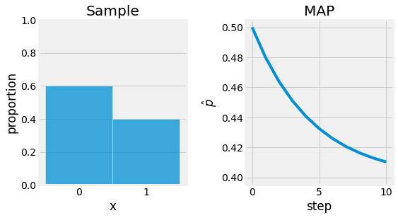
Fig. 4.6 Maximum a Posteriori Estimate applied to the basket ball throw example. The objective is to find \(p\) for \(B(n, p)\). Sample is represented left, and the optimization process base on the MAP right.
Note
Note that if we do not care about the posterior’s argmax but the posterior distribution itself, this is what we refer to as Bayesian Inference. It is the action of guessing in the style of Thomas Bayes. Baye’s style of guessing captures the common sense of knowledge to make better guesses. MAP is, in that sense, only capturing the first mode of the posterior distribution.
4.4.2. Interval Estimates
Until this section, we have only discussed point estimators. But what about Intervals? In this section we study Interval Estimation for the means and for proportions.
4.4.2.1. Interval Estimation of an Expected Value
4.4.2.1.1. With Known Variance
Consider a sample \(X_1, \dots, X_n\), independent and sampled from the same distribution, for example \(\mathcal{N}(\mu, \sigma^2)\) with \(\mu\) unknown and \(\sigma^2\) known. What are the possible value, believable values of \(\sigma\) given our random sample?
We are interested on knowing what the distribution \(\bar{X}\) looks like. Using MLE, we can apporximate this dsitribution:
We also know from the central limit theorem that its standardized centered and reduced form follows a normal distribution when considering a big enough sample size:
from scipy.stats import norm


confidence = 0.95
za = norm.ppf((1 - confidence) / 2)
zb = norm.ppf((1 + confidence) / 2)

print(f"Za = {za:.2f}")
print(f"Zb =  {zb:.2f}")
Za = -1.96
Zb =  1.96
import matplotlib.pyplot as plt
import numpy as np
plt.ion()
plt.style.use("fivethirtyeight")

fig = plt.figure(figsize=(8, 4),  facecolor="white")
ax = fig.add_subplot(1, 1, 1)

X = np.linspace(-4, 4)
ax.plot(X, norm.pdf(X))
ax.axvline(-1.96, linestyle="--", color="r")
ax.axvline( 1.96, linestyle="--", color="g")

X = np.linspace(-1.96, 1.96)
ax.fill_between(X, norm.pdf(X), alpha=0.2)

X = np.linspace(-4, -1.96)
ax.fill_between(X, norm.pdf(X), alpha=0.2, color="r")
X = np.linspace(1.96, 4)
ax.fill_between(X, norm.pdf(X), alpha=0.2, color="g")

ax.text(
    0, 0.10, r"$1 - \alpha$", horizontalalignment='center', verticalalignment='center',
    fontsize=18, color="#008FD5", weight="bold",
)
ax.text(
    -2.5, 0.10, r"$-z_{\alpha / 2}$", horizontalalignment='center', verticalalignment='center',
    fontsize=18, color="#F6424C", weight="bold",
)
ax.text(
    2.5, 0.10, r"$z_{\alpha / 2}$", horizontalalignment='center', verticalalignment='center',
    fontsize=18, color="#328008", weight="bold",
)

fig.subplots_adjust(hspace=0.25, wspace=0.40)
fig.canvas.draw()
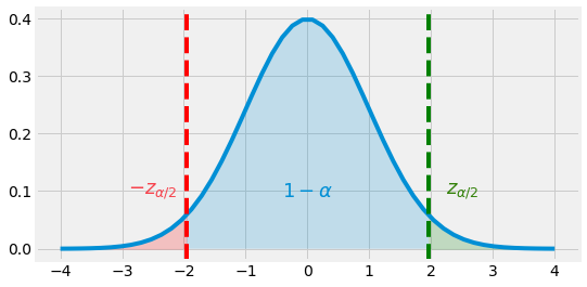
Fig. 4.7 Normal Distribution \(\mathcal{N}(0, 1)\) and \(95\)% range \([-Z_{\alpha / 2}, Z_{\alpha / 2}]\)
If we want to define a \(95\)% Interval Estimate of \(\mu\), for example, we can refer to the normal distribution graph or table and see that it corresponds to area under the curve within the range \([-1.96, 1.96]\). Whe can then say that:
We can now say that the random interval \(\bar{X} \pm 1.96 \sigma / \sqrt{n}\) is a \(95\)% Confidence Interval (CI) for \(\mu\). \(95\)% is reffered to as the Confidence Level, and states that \(P(\mu \in CI) = 1 - \alpha\), with \(alpha\) the Significance Level.
4.4.2.1.2. With Unknown Variance
Let reconsider the same framework but this times without knowing \(\sigma^2\). Our best estimation of the variance is \(S_n^{*2}\) and Fisher’s Theorem telles us that \(\frac{n-1}{\sigma^2} S_n^{*2} \sim \chi_{n-1}^2\). We can then define the Student Statistic:
from scipy.stats import t


confidence = 0.95
ta = t.ppf((1 - confidence) / 2, 9)
tb = t.ppf((1 + confidence) / 2, 9)

print(f"Ta = {ta:.2f}")
print(f"Tb =  {tb:.2f}")
Ta = -2.26
Tb =  2.26
import matplotlib.pyplot as plt
import numpy as np
plt.ion()
plt.style.use("fivethirtyeight")

fig = plt.figure(figsize=(8, 4),  facecolor="white")
ax = fig.add_subplot(1, 1, 1)

X = np.linspace(-4, 4)
ax.plot(X, t.pdf(X, 9))
ax.axvline(-2.26, linestyle="--", color="r")
ax.axvline( 2.26, linestyle="--", color="g")

X = np.linspace(-4, 4)
ax.fill_between(X, t.pdf(X, 9), alpha=0.2)

X = np.linspace(-4, -2.26)
ax.fill_between(X, t.pdf(X, 9), alpha=0.2, color="r")
X = np.linspace(2.26, 4)
ax.fill_between(X, t.pdf(X, 9), alpha=0.2, color="g")

ax.text(
    0, 0.10, r"$1 - \alpha$", horizontalalignment='center', verticalalignment='center',
    fontsize=18, color="#008FD5", weight="bold",
)
ax.text(
    -3, 0.10, r"$-t_{9,\alpha / 2}$", horizontalalignment='center', verticalalignment='center',
    fontsize=18, color="#F6424C", weight="bold",
)
ax.text(
    3, 0.10, r"$t_{9,\alpha / 2}$", horizontalalignment='center', verticalalignment='center',
    fontsize=18, color="#328008", weight="bold",
)

fig.subplots_adjust(hspace=0.25, wspace=0.40)
fig.canvas.draw()
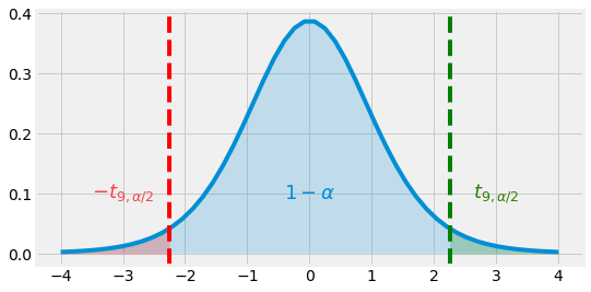
Fig. 4.8 Student Distribution \(T_9\) and \(95\)% range \([-t_{9, \alpha / 2}, t_{9, \alpha / 2}]\)
As we want to obtain a confidence interval for \(\mu\):
We can finally say that \(\bar{X} \pm t_{n-1} \frac{S^*}{\sqrt{n}}\) is a \(95\)% Confidance Interval for \(\mu\).
4.4.2.2. Interval Estimation of a Proportion
A similar approach to the one discussed for the interval estimation of a mean can be applied to estimating an interval for a Proportion. Consider a Binomial test with \(n\) large and let \(X\) denote the number of successes where \(p\), the probability of one success is unknown.
The central limit theorem tells us that:
In that regard, if we want to define a \(100(1 - \alpha)\)% confidence interval:
4.5. Hypothesis Testing
Statistics are great tools for Hypothesis Testing, verifying assumptions, claims, and beliefs based on a data sample. Every hypothesis testing is performed following the given steps:
State a Hypothesis
Select appropriate Test Statistic
Specify the Significance Level
State the Decision Rule regarding the hypothesis
Compute the Sample Statistic
Conclude on the hypothesis
Note
Different statistics and different test types are chosen depending on the study’s framework. A few of them are discussed throughout this chapter. However, the majority of those tests follow the same kind of method.
4.5.1. One-Sample Testing
The first step of hypothesis testing is to formulate what is referred to as the Null and the Alternative hypothesis. The Null Hypothesis \(H_0\) denotes the statement, the population parameter subject to the test. The Alternative Hypothesis \(H_1\), is the opposite statement. If we have enough evidence to reject the null hypothesis, the alternative hypothesis cannot be rejected and assumed to be true. If we do not, the alternative hypothesis is therefore rejected. The following are plosible respectively null and alternative hypothesis:
Note
The belief we want to test, the hypothesis, is \(H_1\). By refuting \(H_0\), we can say we have enough evidence not to deny \(H_1\).
import matplotlib.pyplot as plt
import numpy as np
plt.ion()
plt.style.use("fivethirtyeight")

fig = plt.figure(figsize=(8 * 3, 4),  facecolor="white")
ax2, ax1, ax3 = [fig.add_subplot(1, 3, i + 1) for i in range(3)]

X = np.linspace(-4, 4)
ax1.plot(X, t.pdf(X, 9))
ax2.plot(X, t.pdf(X, 9))
ax3.plot(X, t.pdf(X, 9))

ax1.axvline(0, linestyle="--", color="k")
ax2.axvline(0, linestyle="--", color="k")
ax3.axvline(0, linestyle="--", color="k")

ax1.axvline(-2.26, linestyle="--", color="#008FD5")
ax2.axvline(-1.83, linestyle="--", color="#008FD5")

ax1.axvline( 2.26, linestyle="--", color="#008FD5")
ax3.axvline( 1.83, linestyle="--", color="#008FD5")

X = np.linspace(-4, 4)
ax1.fill_between(X, t.pdf(X, 9), alpha=0.2)
ax2.fill_between(X, t.pdf(X, 9), alpha=0.2)
ax3.fill_between(X, t.pdf(X, 9), alpha=0.2)

X = np.linspace(-4, -2.26)
ax1.fill_between(X, t.pdf(X, 9), alpha=0.4, color="#008FD5")
X = np.linspace(-4, -1.83)
ax2.fill_between(X, t.pdf(X, 9), alpha=0.4, color="#008FD5")

X = np.linspace(2.26, 4)
ax1.fill_between(X, t.pdf(X, 9), alpha=0.4, color="#008FD5")
X = np.linspace(1.83, 4)
ax3.fill_between(X, t.pdf(X, 9), alpha=0.4, color="#008FD5")

ax1.set_axis_off()
ax2.set_axis_off()
ax3.set_axis_off()

ax1.title.set_text("Two-Tailed")
ax2.title.set_text("One-Tailed")
ax3.title.set_text("One-Tailed")


fig.subplots_adjust(hspace=0.25, wspace=0.25)
fig.canvas.draw()
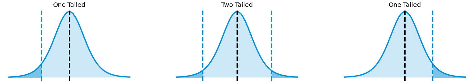
Fig. 4.9 One-Tailed and Two-Tailed satistic test.
A Test Statistic is a quantity computed given a sample. Its value is responsible for deciding whether or not the null hypothesis is rejected. The Z-statistic, the t-statistic, and the chi-statistic are examples of such test statistics. It is often presented in the following form:
After defining this statistic, by considering the region that is consistent with \(H_0\) and the region which is not, the Critical Region, we can compare its value and observe in which of those regions it is found. This allows us to conclude. The value that allows to validate or reject the hypothesis is \(\alpha\) called the Significance. It represented the probability of rejecting the null hypothesis when it is, in fact, true. This value need to be set before computing any value and cannot be changed during and after the test.
For a Left One-Tailed Test:
For a Right One-Tailed Test:
For a Two-Tailed Test:
The Power of a test is given by \(1-\beta\) where \(\beta\) is the significance of \(H_1\).
Let us consider some examples:
Two-Tailed Test:
A factory is responsible for manufacturing M4 screws. An employee believes the average socket-head cap diameter is not \(3\) mm. Using 45 samples, they measure the average diameter produced by their machine and found \(2.8\) mm with plus or minus \(0.15\) mm.
In this problem, we can define:
Let us choose a confidence of \(95\)%. In this case, as the sample size is greater than \(30\), we can call the Central Limit Theorem and use the Z-statistic.
import matplotlib.pyplot as plt
import numpy as np
plt.ion()
plt.style.use("fivethirtyeight")

fig = plt.figure(figsize=(8, 4),  facecolor="white")
ax = fig.add_subplot(1, 1, 1)

X = np.linspace(-4, 4)
ax.plot(X, norm.pdf(X))
ax.axvline(-1.96, linestyle="--", color="#008FD5")
ax.axvline( 1.96, linestyle="--", color="#008FD5")
ax.axvline((2.8 - 3.0) / (0.15 / np.sqrt(45)), linestyle="--", color="#F6424C")

X = np.linspace(-1.96, 1.96)
ax.fill_between(X, norm.pdf(X), alpha=0.2)

X = np.linspace(-4, -1.96)
ax.fill_between(X, norm.pdf(X), alpha=0.4, color="#008FD5")
X = np.linspace(1.96, 4)
ax.fill_between(X, norm.pdf(X), alpha=0.4, color="#008FD5")

ax.text(
    0, 0.10, r"$1 - \alpha$", horizontalalignment='center', verticalalignment='center',
    fontsize=18, color="#008FD5", weight="bold",
)
ax.text(
    -2.5, 0.10, r"$-z_{\alpha / 2}$", horizontalalignment='center', verticalalignment='center',
    fontsize=18, color="#008FD5", weight="bold",
)
ax.text(
    2.5, 0.10, r"$z_{\alpha / 2}$", horizontalalignment='center', verticalalignment='center',
    fontsize=18, color="#008FD5", weight="bold",
)
ax.text(
    -8.5, 0.10, r"$z_c$", horizontalalignment='center', verticalalignment='center',
    fontsize=18, color="#F6424C", weight="bold",
)

fig.subplots_adjust(hspace=0.25, wspace=0.40)
fig.canvas.draw()
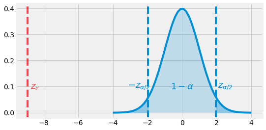
Fig. 4.10 Two-Tailed example. The Z-value is in the rejection zone.
Looking at the \(\mathcal{N}(0, 1)\) pdf, we can observe that our statistic value \(z_c\) is lower than \(-z_{0.025} = -1.96\). It is positioned in the rejection zone. In this case, we can reject the null hypothesis and conclude that with a \(95\)% confidence, the machine does not hold.
Left One-Tailed Test:
A company is manufacturing light bulbs with an average lifespan of \(1.5k\) hours. An engineer believes this value to be less. Using 15 samples, he measures the average lifespan to be \(1.1k\) hours with a standard deviation of \(0.12k\).
In this problem, we can define:
Let us consider a confidence of \(99\)%. There are less than 30 samples, and the population standard deviation is unknown. We will then use a t-statistic:
import matplotlib.pyplot as plt
import numpy as np
plt.ion()
plt.style.use("fivethirtyeight")

fig = plt.figure(figsize=(8, 4),  facecolor="white")
ax = fig.add_subplot(1, 1, 1)

X = np.linspace(-4, 4)
ax.plot(X, norm.pdf(X))
ax.axvline(-t.ppf(0.99, 14), linestyle="--", color="#008FD5")
ax.axvline((1.1 - 1.5) / (0.12 / np.sqrt(15)), linestyle="--", color="#F6424C")

X = np.linspace(-t.ppf(0.99, 14), 4)
ax.fill_between(X, norm.pdf(X), alpha=0.2)

X = np.linspace(-4, -t.ppf(0.99, 14))
ax.fill_between(X, norm.pdf(X), alpha=0.4, color="#008FD5")

ax.text(
    0, 0.10, r"$1 - \alpha$", horizontalalignment='center', verticalalignment='center',
    fontsize=18, color="#008FD5", weight="bold",
)
ax.text(
    -4.5, 0.10, r"$-t_{\alpha, n-1}$", horizontalalignment='center', verticalalignment='center',
    fontsize=18, color="#008FD5", weight="bold",
)
ax.text(
    -11.5, 0.10, r"$t_c$", horizontalalignment='center', verticalalignment='center',
    fontsize=18, color="#F6424C", weight="bold",
)

fig.subplots_adjust(hspace=0.25, wspace=0.40)
fig.canvas.draw()
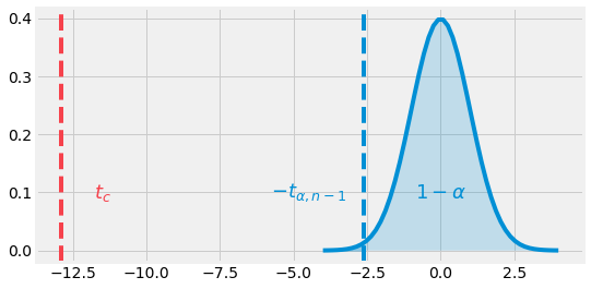
Fig. 4.11 Left One-Tailed example. The t-value is in the rejection zone.
By looking a the pdf of a t-distribution with \(n-1\) degrees of freedom (df), we can observe our statistic value is way lower than the critical value \(t_{0.01, 14} = -2.62\). In this sense, we can reject the null hypothesis with a confidence of \(99\)%.
4.5.2. Two-Sample Testing
Hypothesis testing does not always infer belief in one unique sample. You may want to compare and assess the belief between two different samples. This is what Two-Sample Testing is designed for. A two-sample test can be transformed into a one-sample test by applying a simple trick. Let us consider an example.
Consider two basketball teams. Team A claims that their players have a number of 3 points field goals significantly different than team B. During the season, team A has \(15\) players and yield a mean of \(35\) with a standard deviation of \(5.2\) per player, against \(13\) players for team B with a mean of \(28\) and a standard deviation of \(3.7\). Is there a significant difference between the two teams? Let us consider a \(95\)% confidence.
In this problem we can define:
Given the lower sample size, we consider a t-statistic with degrees of freedom given by:
The statistic value for this test needs to be less than \(-t_{0.025, 9}\) or greater than \(t_{0.025, 9}\) to be rejected with \(t_{0.025, 9} \approx -2.26\).
We can now conclude that there is a significant difference at \(5\)% between the two teams.
4.5.3. P-Value Method
The P-Value method is commonly used to decide on the rejection of the null hypothesis. It is an extension of the methods presented above. Instead of just considering the statistic position compared to the critical value of a given significance level, we consider the hole rejection area. This rejection area corresponds to the probability of rejecting the null hypothesis with a given significance level. The new decision rule is then:
Let us reuse the example of the one-sample left one-tailed test with the light bulb life span. By referring to a \(\text{p-value}\) table of a t-distribution with \(14\) degrees of freedom, we find that \(\text{p-value}=1.8\times10^{-9}\) which is way lower than \(\alpha=0.05\). We can then conclude that H_0 is rejected with a confidence of \(95\)%.
from scipy.stats import t

import numpy as np


t_stat = (1.1 - 1.5) / (0.12 / np.sqrt(15))
p_value = t.sf(np.abs(t_stat), 14)             # times 2 for two-tailed tests

print(f"t-statistic: {t_stat:.2f}")
print(f"p-value    : {p_value:.2g}")
t-statistic: -12.91
p-value    : 1.8e-09
4.5.4. Hypthesis Tests Zoo
Here is a non-exhaustive table of Hypothesis Tests:
Data Type |
Variable |
One-Sample |
Two-Sample |
Multi-Sample |
|---|---|---|---|---|
Continuous & Normality assumption |
\(\mu\) |
\(\begin{align}H_0&:\;\mu=\mu_0 \\ H_1&:\;\mu\neq\mu_0\end{align}\\\textbf{T-Test}\) |
\(\begin{align}H_0&:\;\mu_0=\mu_2 \\ H_1&:\;\mu_0\neq\mu_1\end{align}\\\textbf{T-Test}\) |
\(\begin{align}H_0&:\;\mu_0=\dots=\mu_k \\ H_1&:\;\text{At least one mean is different}\end{align}\\\textbf{Analysis of Variance}\) |
Continuous & Normality assumption |
\(\sigma\) |
\(\begin{align}H_0&:\;\sigma=\sigma_0 \\ H_1&:\;\sigma\neq\sigma_0\end{align}\\\textbf{Chi-Square Test}\) |
\(\begin{align}H_0&:\;\sigma_0=\sigma_2 \\ H_1&:\;\sigma_0\neq\sigma_1\end{align}\\\textbf{F-Test}\) |
\(\begin{align}H_0&:\;\sigma_0=\dots=\sigma_k \\ H_1&:\;\text{One is different}\end{align}\\\textbf{Bartlett's Test}\) |
Continuous & Non Normal |
\(\eta\) |
\(\begin{align}H_0&:\;\eta=\eta_0 \\ H_1&:\;\eta\neq\eta_0\end{align}\\\textbf{Wilcoxon Test}\) |
\(\begin{align}H_0&:\;\eta_0=\eta_2 \\ H_1&:\;\eta_0\neq\eta_1\end{align}\\\textbf{Mann-Whitney Test}\) |
\(\begin{align}H_0&:\;\eta_0=\dots=\eta_k \\ H_1&:\;\text{One is different}\end{align}\\\textbf{Kruskal-Wallis Test}\) |
Discrete |
\(\pi\) |
\(\begin{align}H_0&:\;\pi=\pi_0 \\ H_1&:\;\pi\neq\pi_0\end{align}\\\textbf{Proportion Test}\) |
\(\begin{align}H_0&:\;\pi_0=\pi_2 \\ H_1&:\;\pi_0\neq\pi_1\end{align}\\\textbf{Proportion Test}\) |
\(\begin{align}H_0&:\;\pi_0=\dots=\pi_k \\ H_1&:\;\text{One is different}\end{align}\\\textbf{Binomial Analysis of Means}\) |
4.6. Applications
Statistical Inference and Probabilities are key to Machine and Deep Learning, and Applied Mathematics in general. This section details common uses of those concepts especially to the use of Machine Learning.
4.6.1. Linear VS Logistic Regression
Let us consider the Breast Cancer Dataset example for PCA in the Linear Algebra Chapter. To simplify the explanations, we apply PCA on the features to obtain only one feature, the projection on to the first principal component, capturing most variation. As a reminder our goald with this dataset is to classify a person as having a breast cancer \(1\) or not \(0\).
from sklearn.datasets import load_breast_cancer
from sklearn.model_selection import train_test_split
from sklearn.preprocessing import StandardScaler

import pandas as pd
pd.set_option("display.max_columns", 8)


# To Normalize Data (Mean Center and Normalize Variation)
sc = StandardScaler()

# Load Breast Cancer dataset in memory
data = load_breast_cancer(return_X_y=False)
X, y = sc.fit_transform(data.data), data.target

# Split Dataset
X_train, X_test, y_train, y_test = train_test_split(X, y, test_size=0.33, random_state=42)

# Show data as a dataframe to display infos table
df = pd.DataFrame(data=X, columns=data.feature_names)
df.head()
| mean radius | mean texture | mean perimeter | mean area | ... | worst concavity | worst concave points | worst symmetry | worst fractal dimension | |
|---|---|---|---|---|---|---|---|---|---|
| 0 | 1.097064 | -2.073335 | 1.269934 | 0.984375 | ... | 2.109526 | 2.296076 | 2.750622 | 1.937015 |
| 1 | 1.829821 | -0.353632 | 1.685955 | 1.908708 | ... | -0.146749 | 1.087084 | -0.243890 | 0.281190 |
| 2 | 1.579888 | 0.456187 | 1.566503 | 1.558884 | ... | 0.854974 | 1.955000 | 1.152255 | 0.201391 |
| 3 | -0.768909 | 0.253732 | -0.592687 | -0.764464 | ... | 1.989588 | 2.175786 | 6.046041 | 4.935010 |
| 4 | 1.750297 | -1.151816 | 1.776573 | 1.826229 | ... | 0.613179 | 0.729259 | -0.868353 | -0.397100 |
5 rows × 30 columns
df.info()
<class 'pandas.core.frame.DataFrame'>
RangeIndex: 569 entries, 0 to 568
Data columns (total 30 columns):
 #   Column                   Non-Null Count  Dtype
---  ------                   --------------  -----
 0   mean radius              569 non-null    float64
 1   mean texture             569 non-null    float64
 2   mean perimeter           569 non-null    float64
 3   mean area                569 non-null    float64
 4   mean smoothness          569 non-null    float64
 5   mean compactness         569 non-null    float64
 6   mean concavity           569 non-null    float64
 7   mean concave points      569 non-null    float64
 8   mean symmetry            569 non-null    float64
 9   mean fractal dimension   569 non-null    float64
 10  radius error             569 non-null    float64
 11  texture error            569 non-null    float64
 12  perimeter error          569 non-null    float64
 13  area error               569 non-null    float64
 14  smoothness error         569 non-null    float64
 15  compactness error        569 non-null    float64
 16  concavity error          569 non-null    float64
 17  concave points error     569 non-null    float64
 18  symmetry error           569 non-null    float64
 19  fractal dimension error  569 non-null    float64
 20  worst radius             569 non-null    float64
 21  worst texture            569 non-null    float64
 22  worst perimeter          569 non-null    float64
 23  worst area               569 non-null    float64
 24  worst smoothness         569 non-null    float64
 25  worst compactness        569 non-null    float64
 26  worst concavity          569 non-null    float64
 27  worst concave points     569 non-null    float64
 28  worst symmetry           569 non-null    float64
 29  worst fractal dimension  569 non-null    float64
dtypes: float64(30)
memory usage: 133.5 KB
from sklearn.decomposition import PCA


pca = PCA(n_components=1).fit(X_train)
pca_X_train = pca.fit_transform(X_train)
pca_X_test = pca.fit_transform(X_test)
import matplotlib.pyplot as plt
plt.ion()
plt.style.use('fivethirtyeight')


def plot_data(ax: plt.Figure, pca_X: np.ndarray, y: np.ndarray) -> None:
    lc, ln = False, False    # Ensure only one label for legend
    for coord, label in zip(pca_X, y):
        c = "r" if label else "#008FD5"
        m = "<" if label else "o"

        l = "Cancer" if label else "Normal"
        if l == "Cancer" and not lc: lc = True
        elif l == "Normal" and not ln: ln = True
        else: l = "_"

        ax.scatter(coord, label, color=c, marker=m, alpha=0.5, label=l)
    ax.set_xlabel("PCA 1")
    ax.set_ylabel("probability of breast cancer")
    ax.legend()


fig = plt.figure(figsize=(4, 4), facecolor="white")
ax = fig.add_subplot(1, 1, 1)

plot_data(ax, pca_X_train, y_train)

fig.canvas.draw()
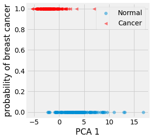
Fig. 4.12 Visualization of the firs principal axis against the probability of having a breast cancer for the training data.
As a first step, we can observe that the random variable \(Y\) we are studying, the probability of a patient with breast cancer or not, is binary and follows a Bernoulli distribution \(B(p)\). We are interested in estimating the parameter \(p\) of that distribution given our dataset.
In this example, we wan to find a model that gives us this probability given a data point, patient features, or feature in this case:
If there is a linear between X and Y, we can use a Linear Regression as presented in the Linear Algebra Chapter. As a reminder, here is the definition of a linear model applied to our study case:
One problem with such a formulation is that \(p(x)\) can take negative values and positive values above 1. This cannot happened for probabilities. One way to fix this issue is to constrain this model by applying a monolitic function that maps \(z = \beta_0 + \beta_1 x\) to the \([0, 1]\) range. The sigmoid function, sometimes called the logistic function, is such a function:
import matplotlib.pyplot as plt
import numpy as np
plt.ion()
plt.style.use('fivethirtyeight')

fig = plt.figure(figsize=(4, 4), facecolor="white")
ax = fig.add_subplot(1, 1, 1)

X = np.linspace(-10, 10, 100)
sigmoid = lambda z: 1 / (1 + np.exp(-z))
ax.plot(X, sigmoid(X))
ax.set_xlabel("x")
ax.set_ylabel("y")

fig.canvas.draw()
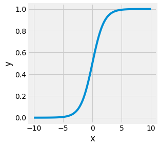
Fig. 4.13 Sigmoid function.
We are now performing what is called Logistic Regression. The probability of a given data point to correspond to a patient with breast cancer is now given by:
This equation can be rewritten as follow:
The left factor is referred to as the logits, or log-odds, and the internal log factor as the odds. It is now just a matter of fitting a line into the logits projection, in other world estimating the coefficients \(\beta_0\) and \(\beta_1\). This can be achieved using the MLE.
As a reminder, maximizing the likelihood is the same as maximizing the log-likelihood:
Note
Note that minimizing the negative loglikelihood is equivalent to minimizing the cross-entropy defined by Shannon, in this case the binary cross-entropy.
from torch.optim import SGD

import numpy as np
import torch
import torch.nn as nn
np.random.seed(42)
torch.manual_seed(42)


class LinearRegression(nn.Module):
    def __init__(self) -> None:
        super(LinearRegression, self).__init__()
        self.linear = nn.Linear(1, 1)

    def forward(self, x: torch.Tensor) -> torch.Tensor:
        return self.linear(x)

    def fit(self, X: torch.Tensor, y: torch.Tensor, lr: float = 1e-3, iterations: int = 100) -> float:
        criterion = nn.MSELoss()
        optimizer = SGD(self.parameters(), lr=lr)
        self.train()

        for i in range(iterations):
            optimizer.zero_grad()
            y_pred = self(X)
            loss = criterion(y_pred, y)
            loss.backward()
            optimizer.step()
        acc = ((y_pred > 0.5) == y).float().sum() / len(X) * 100
        print(f"[Train] Linear   Regression [{i+1}/{iterations}] acc:{acc.item():.2f}%")


class LogisticRegression(nn.Module):
    def __init__(self) -> None:
        super(LogisticRegression, self).__init__()
        self.linear = nn.Linear(1, 1)

    def forward(self, x: torch.Tensor) -> torch.Tensor:
        logits = self.linear(x)
        return torch.sigmoid(logits)

    def fit(self, X: torch.Tensor, y: torch.Tensor, lr: float = 1e-3, iterations: int = 100) -> None:
        criterion = nn.BCELoss()
        optimizer = SGD(self.parameters(), lr=lr)
        self.train()

        for i in range(iterations):
            optimizer.zero_grad()
            y_pred = self(X)
            loss = criterion(y_pred, y)
            loss.backward()
            optimizer.step()
        acc = ((y_pred > 0.5) == y).float().sum() / len(X) * 100
        print(f"[Train] Logistic Regression [{i+1}/{iterations}] acc:{acc.item():.2f}%")


linear_reg = LinearRegression()
linear_reg.fit(torch.Tensor(pca_X_train), torch.Tensor(y_train).unsqueeze(1))

logistic_reg = LogisticRegression()
logistic_reg.fit(torch.Tensor(pca_X_train), torch.Tensor(y_train).unsqueeze(1))
[Train] Linear   Regression [100/100] acc:66.40%
[Train] Logistic Regression [100/100] acc:83.20%
X, y = torch.Tensor(pca_X_test), torch.Tensor(y_test).unsqueeze(1)

y_pred = linear_reg(X)
acc = ((y_pred > 0.5) == y).float().sum() / len(X) * 100
print(f"[Test] Linear   Regression acc:{acc.item():.2f}%")

y_pred = logistic_reg(X)
acc = ((y_pred > 0.5) == y).float().sum() / len(X) * 100
print(f"[Test] Logistic Regression acc:{acc.item():.2f}%")
[Test] Linear   Regression acc:70.21%
[Test] Logistic Regression acc:82.98%
import matplotlib.pyplot as plt
plt.ion()
plt.style.use('fivethirtyeight')


def plot_data(ax: plt.Figure, pca_X: np.ndarray, y: np.ndarray) -> None:
    lc, ln = False, False    # Ensure only one label for legend
    for coord, label in zip(pca_X, y):
        c = "r" if label else "#008FD5"
        m = "<" if label else "o"

        l = "Cancer" if label else "Normal"
        if l == "Cancer" and not lc: lc = True
        elif l == "Normal" and not ln: ln = True
        else: l = "_"

        ax.scatter(coord, label, color=c, marker=m, alpha=0.5, label=l)
    ax.set_xlabel("PCA 1")
    ax.set_ylabel("probability of breast cancer")


fig = plt.figure(figsize=(8, 4), facecolor="white")
ax1, ax2 = [fig.add_subplot(1, 2, i + 1) for i in range(2)]

linear_reg.eval()
X = torch.linspace(-6, 16, 100).unsqueeze(1)
plot_data(ax1, pca_X_test, y_test)
ax1.plot(X, linear_reg(X).detach().numpy(), label="Linear", color="#E5AE42")
ax1.legend()
ax1.title.set_text("linear regression")

logistic_reg.eval()
X = torch.linspace(-6, 16, 100).unsqueeze(1)
plot_data(ax2, pca_X_test, y_test)
ax2.plot(X, logistic_reg(X).detach().numpy(), label="Logistic", color="#E5AE42")
ax2.legend()
ax2.title.set_text("logsitic regression")

fig.subplots_adjust(hspace=0.25, wspace=0.40)
fig.canvas.draw()
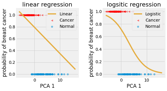
Fig. 4.14 Linear and Logistic Regression on breast cancer PCA 1 test set.
As we can observe from the results, the Logistic Regression is better suited to classification than the Linear one. They respectively yield an \(82.98\)% accuracy on the test set for the logistic regression, against \(70.21\)% for the linear regression.
It is possible to verify the assumption that one model is better than another one by applying our knowledge on hypothesis testing. However, this will not be treated in this chapter.
4.6.2. Naive Bayes Classification
Naive Bayes Classifiers is a family of simple classifiers relying on the Bayes’ Theorem and the independence of the features. In this section, we discuss its use on the problem of Spam Identification.
Let us consider an email, or message \(m\), as an organized sequence of unique words \(w_1, \dots, w_n\). The goal of spam identification can be stated as finding the conditionnal probability of this message beign a spam given all those worlds:
Computing the posterior probability, even without considering the marginal term, gives a direct way to classify a mail as being spam or not. We need to compare the posterior of spam given the words and the posterior of not being spam given those same words—the most significant wins.
Note
Be careful, Naive Bayes Classifiers does not consider the order of the worlds, it only matters about their frequency in conjunction with its class, spam or not.
The common practice is to establish a Bag of Word to consider as a training set. If a word does not appear in the message, its probability is \(0\). The standard is then to add a default value \(\alpha\) to all the worlds’ frequency.
For this application example we will use the SMS Spam Collection Dataset containing \(5,574\) messages tagged as “Spam” or “Ham”.
import pandas as pd


df = pd.read_csv("datasets/sms_spam_dataset.csv", encoding="latin-1")
df = df[["v1", "v2"]].rename(columns={"v1": "label", "v2": "sms"})
df.head()
| label | sms | |
|---|---|---|
| 0 | ham | Go until jurong point, crazy.. Available only ... |
| 1 | ham | Ok lar... Joking wif u oni... |
| 2 | spam | Free entry in 2 a wkly comp to win FA Cup fina... |
| 3 | ham | U dun say so early hor... U c already then say... |
| 4 | ham | Nah I don't think he goes to usf, he lives aro... |
Let us begin by cleaning this dataset and removing all unnecessary features of the English language considering the use of a Naive Bayes Classifier. We first lowercase all the text, remove all the English stop words, punctuation, and special symbols. We can even apply stemming or lemming by reducing the inflection forms of words with the same lemma.
from nltk import stem
from nltk.corpus import stopwords
from nltk.tokenize import word_tokenize

import nltk
# nltk.download('stopwords')
# nltk.download('punkt')


LANGUAGE = "english"

stemmer = stem.SnowballStemmer(LANGUAGE)
stopwords = set(stopwords.words(LANGUAGE))

clean_up = lambda msg: " ".join([
    stemmer.stem(word)
    for word in word_tokenize(msg.lower())
    if word not in stopwords and word.isalpha()
])

df["sms_clean"] = df["sms"].apply(clean_up)
df.head()
| label | sms | sms_clean | |
|---|---|---|---|
| 0 | ham | Go until jurong point, crazy.. Available only ... | go jurong point crazi avail bugi n great world... |
| 1 | ham | Ok lar... Joking wif u oni... | ok lar joke wif u oni |
| 2 | spam | Free entry in 2 a wkly comp to win FA Cup fina... | free entri wkli comp win fa cup final tkts may... |
| 3 | ham | U dun say so early hor... U c already then say... | u dun say earli hor u c alreadi say |
| 4 | ham | Nah I don't think he goes to usf, he lives aro... | nah think goe usf live around though |
One standard way to define the word’s distribution is to build a bag of words and its corresponding frequency table for each document. As the task of spam identification is simple, this may be suited. However, we will use another common word vectorizing technique using the TF-IDF statistic:
from sklearn import metrics
from sklearn.feature_extraction.text import TfidfVectorizer
from sklearn.naive_bayes import MultinomialNB


random_df = df.sample(frac=1, random_state=42)
split = int(len(random_df) * 0.8)

train_df = random_df[:split].reset_index(drop=True)
test_df = random_df[split:].reset_index(drop=True)

vectorizer = TfidfVectorizer()
X_train, y_train = vectorizer.fit_transform(train_df["sms_clean"]), train_df["label"]
X_test, y_test = vectorizer.transform(test_df["sms_clean"]), test_df["label"]

naive_bayes_classifier = MultinomialNB()
naive_bayes_classifier.fit(X_train, y_train)
acc = metrics.accuracy_score(naive_bayes_classifier.predict(X_train), y_train)
print(f"[Train] Naive Bayes, acc: {acc * 100:.2f}%")

acc = metrics.accuracy_score(naive_bayes_classifier.predict(X_test), y_test)
print(f"[Test]  Naive Bayes, acc: {acc * 100:.2f}%")
[Train] Naive Bayes, acc: 97.60%
[Test]  Naive Bayes, acc: 96.23%
We finally obtain a \(96.23\)% accuracy on the test set when applying Naive Bayes Classification with TF-IDF. This result is quite significant and was relatively easy to achieve. Moreover, this method scales linearly with the vocabulary and message’s length. All those reasons make Naive Bayes Classifier a great tool for this kind of task.
Note
The accuracy metric has been used throughout this chapter. This is not the only metric, and it is not sufficient to conclude on a model performance in every case. Other metrics will be discussed in the following chapters.